Week 3 - External flow simulation over an Ahmed body.

AIM: To perform external flow simulation over an Ahmed Body and compare the numerical results with the available experimental data.

OBJECTIVES:

• Ahmed's body and its importance.
• The reason for the negative pressure in the wake region.
• The signification of the point of separation.

EXPECTED RESULTS:

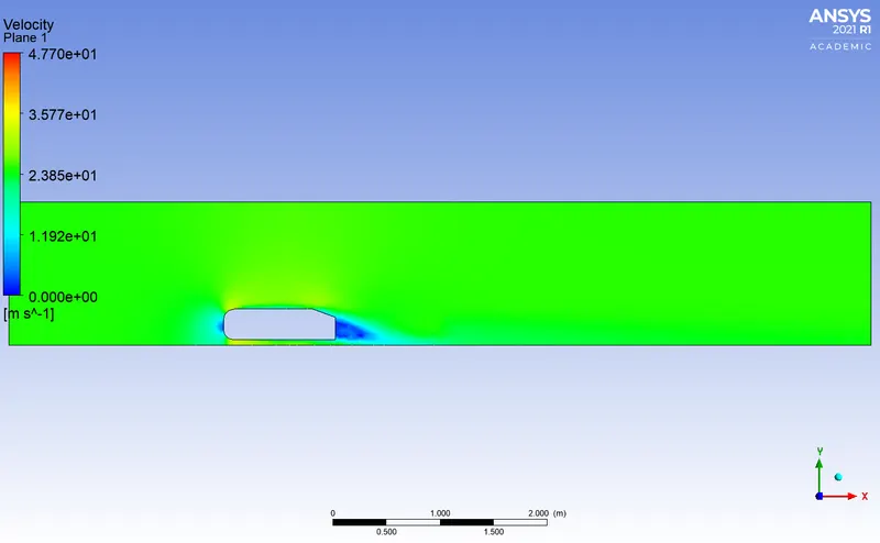
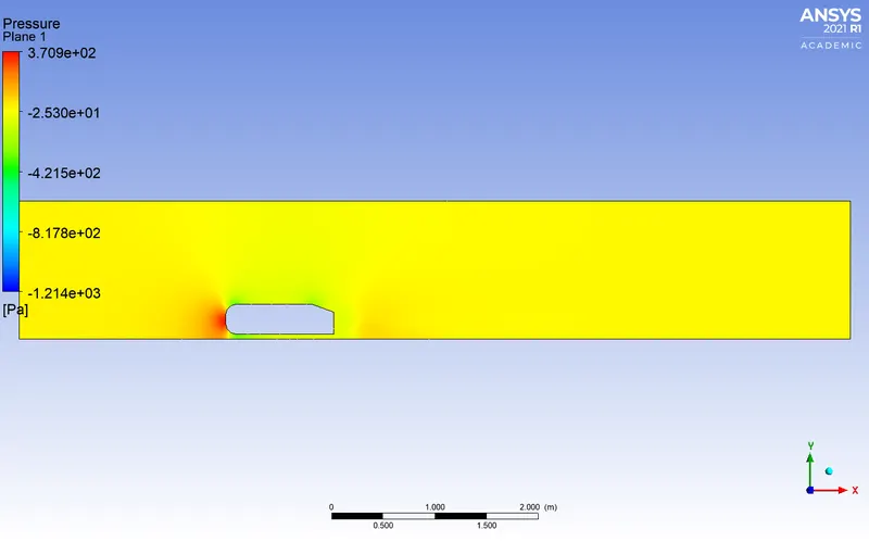
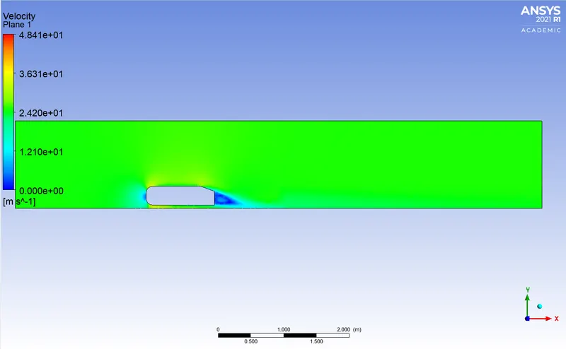
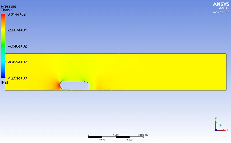
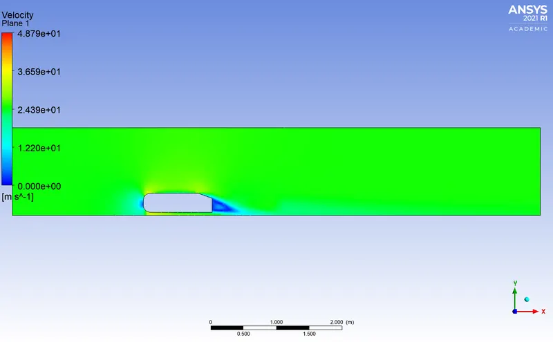
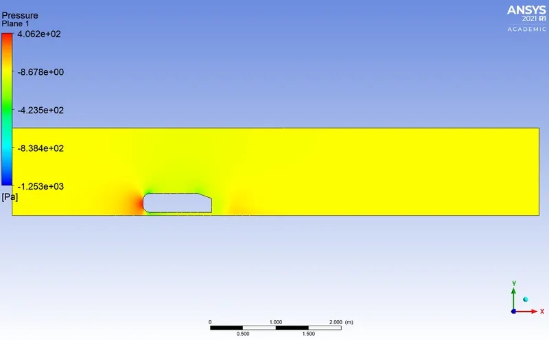
• Velocity and Pressure contours.
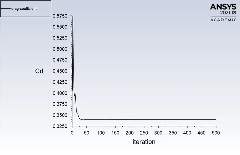
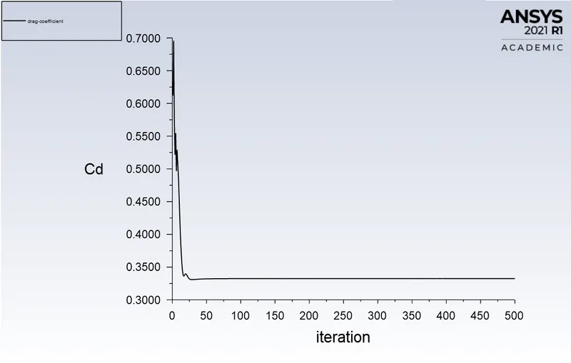
• The drag coefficient plot for a refined case. (For velocity of 25m/sec. the drag coefficient should be around 0.33).
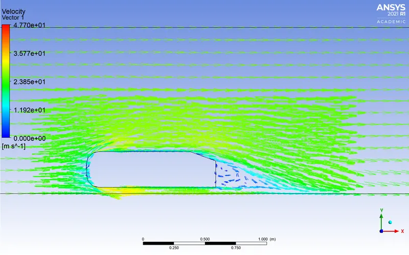
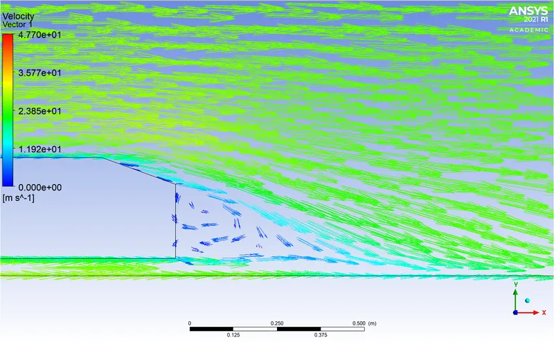
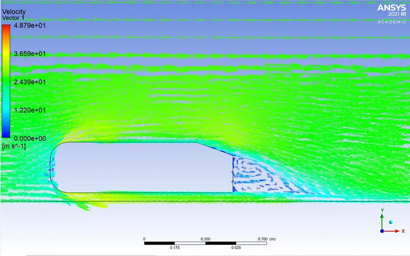
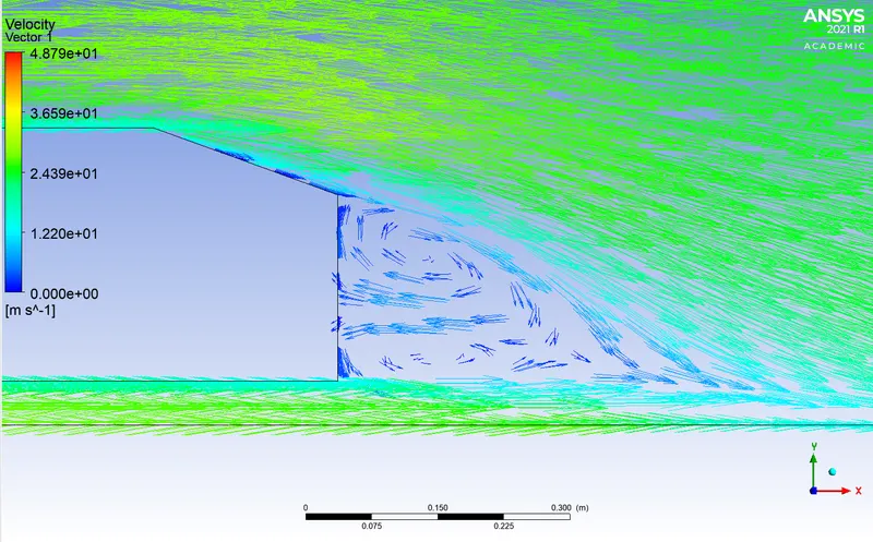
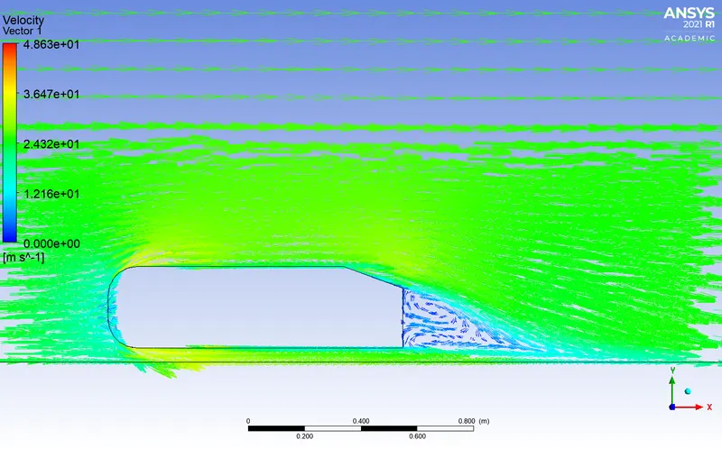
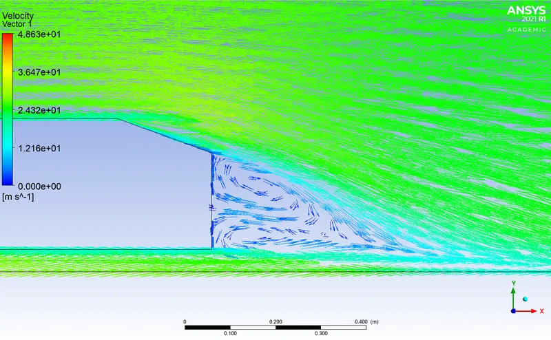
• The vector plot clearly showing the wake region.
• Perform the grid independence test and provide the values of drag and lift with each case.

INTRODUCTION:

CFD simulation is an efficient tool in the automotive industry used extensively for design. This allows the designers to obtain a quick and proper analysis before go-ahead to the final step. Recently, the CFD approach has been adopted effectively within the automotive industry, with several new methods for car design.

CFD analysis in the car industry is used in the determination of the applied forces and that of the vehicle's wake during moving. CFD is also used to analyze the effect of wake on the vehicle's efficiency and capability compared to other cars.

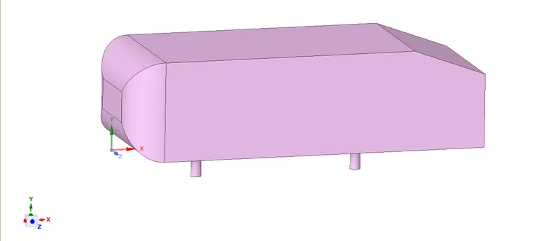
In the vehicle industry, Ahmed Car Body is the standard model used as a validating case in industry and CFD simulation. Ahmed Body is a generic car-type bluff body with a slank back that has different angles from 0-40 degrees. It is usually used as a benchmark test case for simulating the external aerodynamic flow characteristic over a car model.

IMPORTANCE OF THE AHMED BODY:

The Ahmed body is considered a generic car body. This was first defined and characterized in the experimental work. It is a benchmark model that is used in the automotive industry for validating simulation tools since it possesses car-like geometry features. The essential flow features around the geometry are captured by the air flowing around the Ahmed body. It is used to validate the numerical model based on the experimental data from the wind tunnel testing is available for the Ahmed body. The validated numerical model is then used to design new models of the car. It also helps in the study of the effects of various other parameters on the automobile body.

AHMED BODY GEOMETRY:

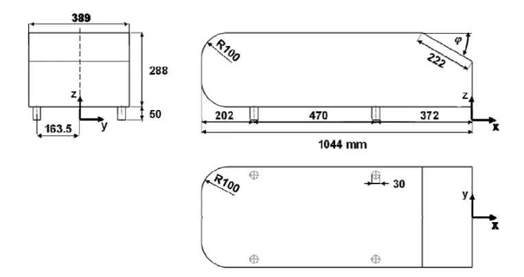
The geometrical shape of the Ahmed body investigated is depicted below figure. Despite the considerable deviation of its geometry from usual vehicles, the body represents the basic aerodynamic properties of a vehicle, especially in the rear part. The slant angle `phi` strongly influences the aerodynamic drag and lift at the back. Both the drag and lift coefficients change abruptly at the angle `phi = 30^o`. Therefore, this angle is called the critical slant angle. The simple geometrical shape has a length of 1044 mm, a height of 288 mm, and a width of 389 mm. It also has 50 mm cylindrical legs attached to the bottom of the body.

AHMED BODY CAD MODEL:

COMPUTATIONAL DOMAIN:

ANSYS software tools (workbench, Design Modular, Meshing tool & Fluent solver) are used to carry out the flow simulation.

Geometry and Enclosure:

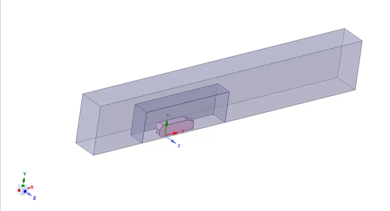
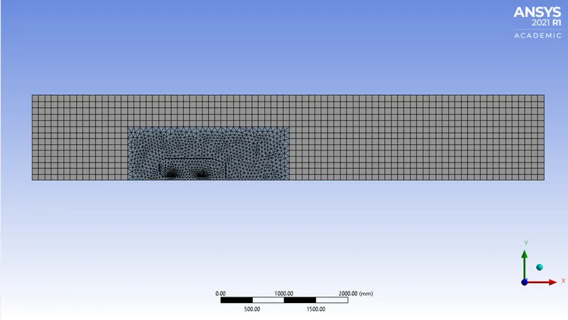
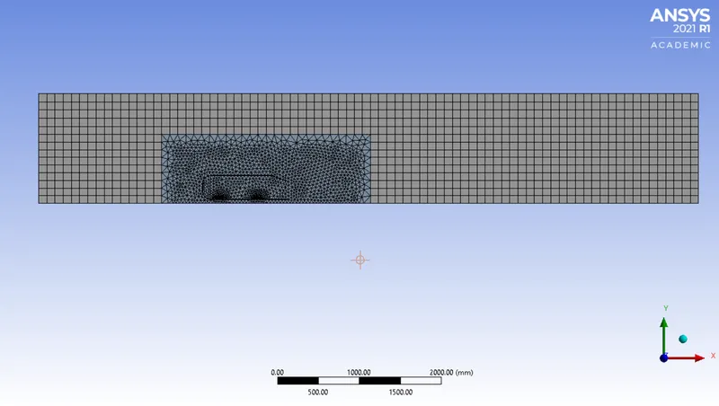
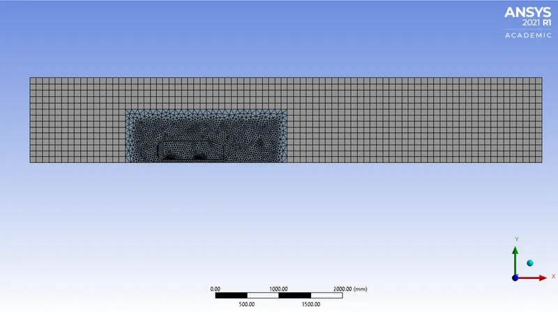
The model was split into half along the XY plane using the split body command in SpaceClaim. Then Two enclosures were made to set up the domain and mesh refinement purposes using the enclosure tool. A smaller enclosure is used around the Ahmed body in order to capture the wake region correctly with a refined mesh in that region.

Meshing:

The length of the first cell away from the surface (y) to calculate effectively the wall shear stress during the simulation should be calculated carefully. To do so, Y+ calculations should be performed to calculate the value of (y) before start the meshing process.

1) Reynolds Number (Re):

`Re = (rhovl)/mu`

`Re = (1.225*25*1.044)/(1.7894e-5)`

`Re = 1786772.102`

2) Skin-Friction Coefficient (Cf):

`Cf = 0.0576*Re^(-0.5)`

`Cf = 0.003236`

3) Wall Shear Stress (`tau_w`):

`tau_w = C_f *1/2rhov^2`

`tau_w = 1.2387` pa

4) Friction Velocity:

`U_t = (tau_w/rho)^0.5`

`U_t = (1.2387/1.225)^0.5`

`U_t = 1.0055` m/s

5) Wall Distance (y):

`y = (y^+ *mu)/(U_t * rho)`

As we will use the K-Epsilon Model - Standard (Range of `Y^+` value is 30-300)

If `Y^+ = 30`

`y = (30*0.000017894)/(1.0055*1.225)`

`y = 0.00043`

`y = 0.43 mm`

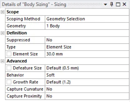
In the mesh window, the faces of the domain are named. The Outer enclosure is mesh using the multizone option in the method to create Hexa mesh. the inner enclosure is mesh using the body sizing option to create tetra mesh.

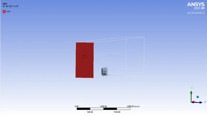
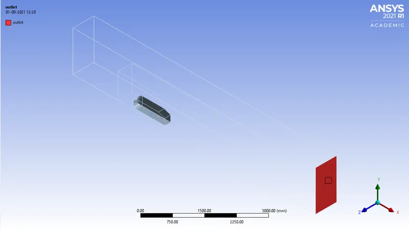
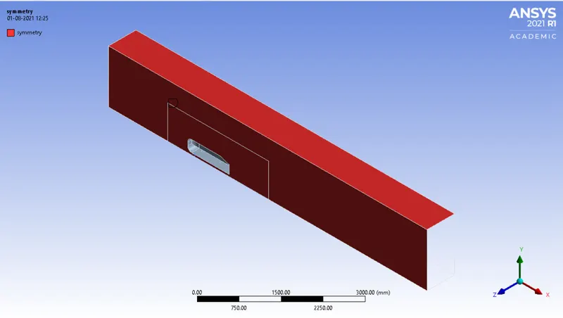
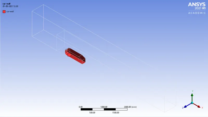
Named Selection:

Inlet

Outlet

Symmetry

Car-wall

Mesh Parameters:

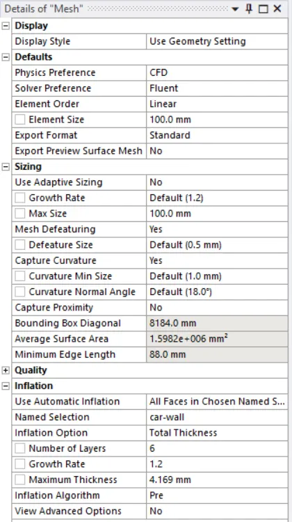
The mesh cell size for the outer domain is 100 mm

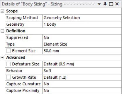
The mesh cell size for the inner domain is 50 mm

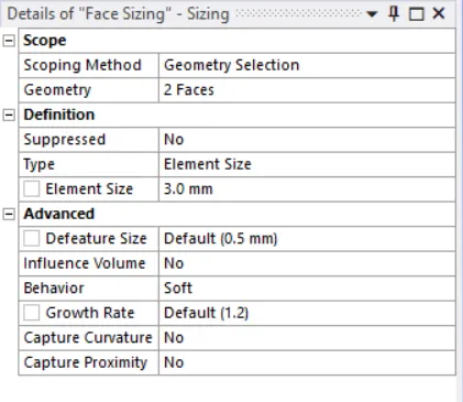
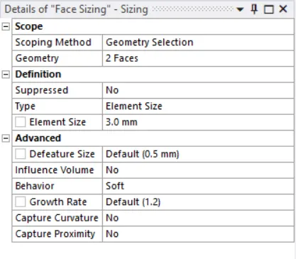
The Ahmed body legs are further refined to an element size of 3 mm.

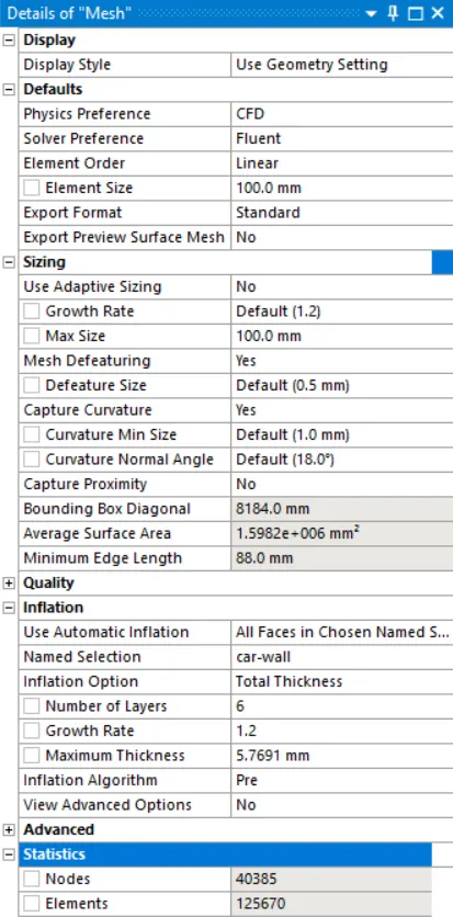
The total number of inflation layers is chosen as 6 with total layer thickness is chosen and its value is 4.169 mm ( when Y+ is 30). the growth rate is 1.2

Mesh

Setup & Solution:

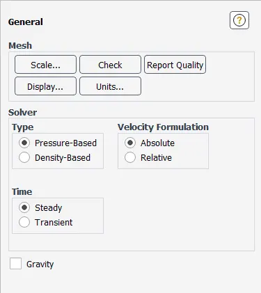
• Solver -> Type -> Pressure-Based, Velocity-Formation -> Absolute, Time -> Steady
• 
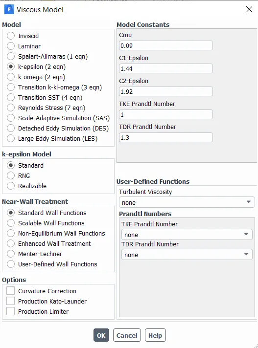
• Viscous -> Model -> k-epsilon, k-epsilon Model -> Standard, Near-Wall Treatment -> Standard Wall Functions, Ok
• 
• Material -> Air
• Boundaries -> Inlet -> Velocity Inlet = 25 m/s, Outlet -> Pressure Outlet -> Gauge pressure = 0
• Solution -> Initialization -> Method -> Hybrid, Initialize.
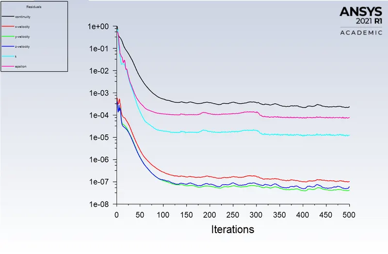
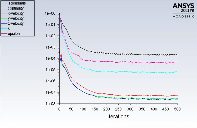
• Run Calculation -> Number of Interations = 500, Calculate.

Results:

Here we have considered a case with a different `Y^+` value with the same mesh size to find appropriate `Y^+` which will give the correct value for the drag coefficient.

Case	Outer enclosure (mm)	Inner enclosure (mm)	`Y^+`	y (mm)	Total Thickness in mm (number of layers 6)	Cd
1	100	50	30	0.43	4.169	0.3482
2	100	50	40	0.5810	5.7691	0.3399
3	100	50	50	0.7263	7.2118	0.3522
4	100	50	100	1.4527	14.4249	0.3545
5	100	50	150	2.1791	21.638	0.3566
6	100	50	200	2.9054	28.8501	0.3571
7	100	50	250	3.6318	36.0632	0.3580
8	100	50	300	4.3582	43.2762	0.3593

From the above table, we can see that the `Y^+= 40` gives Cd = 0.3399, which was our expected value of Cd. So we can use Y+ = 40 for our further cases.

CASE 1.

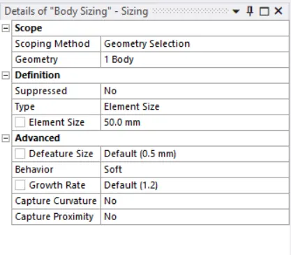
The mesh cell size for the outer domain is 100 mm.

The mesh cell size for the inner domain is 50 mm.

The number of inflation layers is 6 and the total layer thickness is 5.7691 mm

Results:

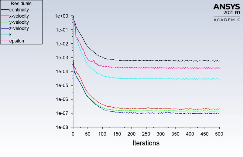
Residual Plot

Drag Coefficient Plot

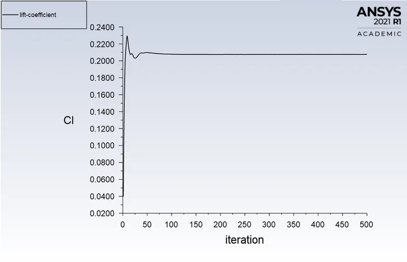
Lift Coefficient Plot

Velocity Contour

Pressure Contour

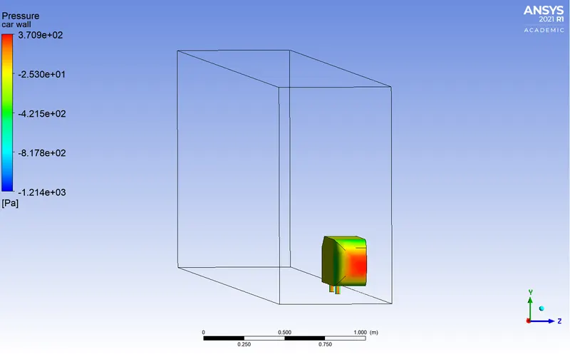
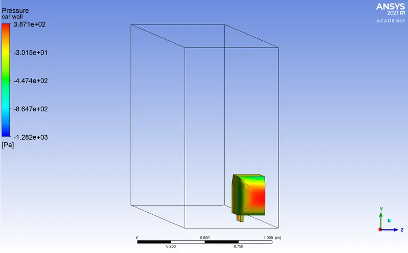
Pressure at car wall

Velocity Vector

CASE 2.

The mesh cell size for the outer domain is 100 mm.

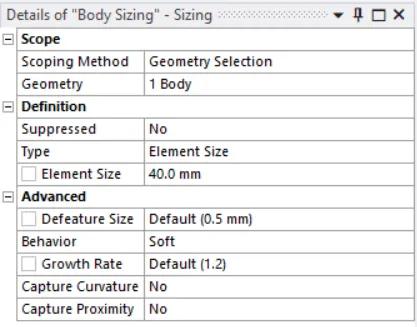
The mesh cell size for the inner domain is 40 mm.

The number of inflation layers is 6 and the total layer thickness is 5.7691 mm

Mesh:

Results:

Residual Plot

Drag Coefficient Plot

Lift Coefficient Plot

Velocity Contour

Pressure Contour

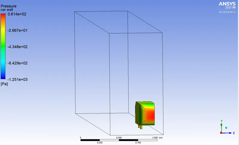
Pressure at Car wall

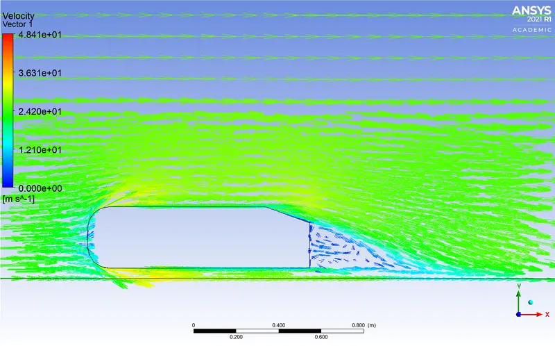
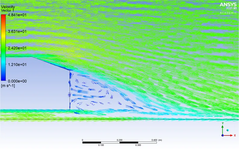
Velocity Vector

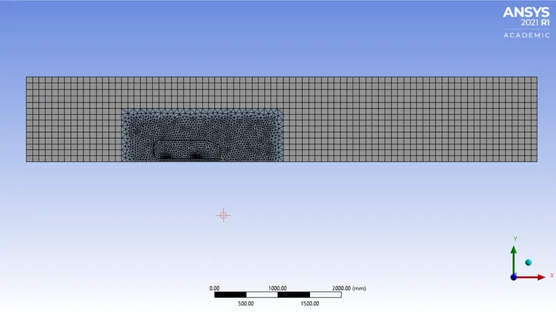
CASE 3.

The mesh cell size for the outer domain is 100 mm.

The mesh cell size for the inner domain is 35 mm.

The number of inflation layers is 6 and the total layer thickness is 5.7691 mm

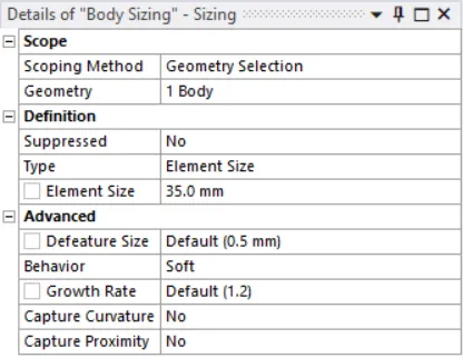
Mesh:

Results:

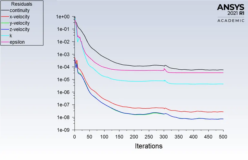
Residual Plot

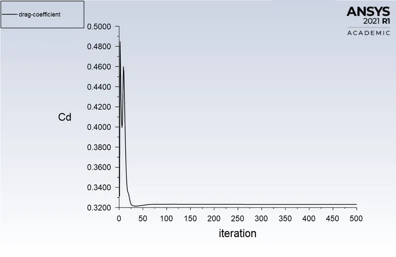
Drag Coefficient Plot

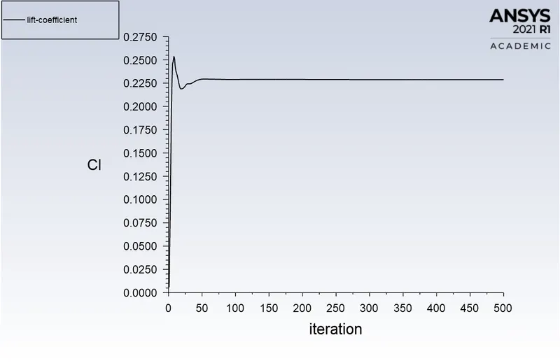
Lift Coefficient Plot

Velocity Contour

Pressure Contour

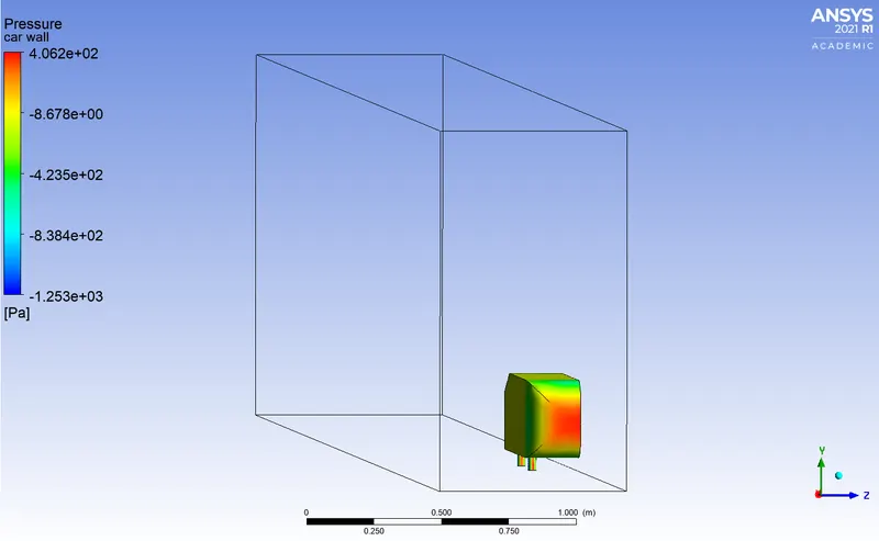
Pressure at Car wall

Velocity Vector

CASE 4.

The mesh cell size for the outer domain is 100 mm.

The mesh cell size for the inner domain is 30 mm.

The number of inflation layers is 6 and the total layer thickness is 5.7691 mm

Mesh:

Results:

Residual Plot

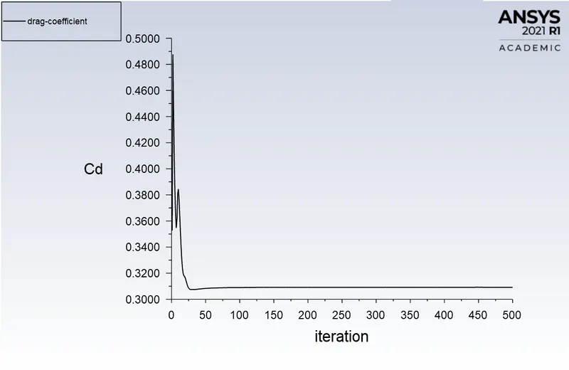
Drag Coefficient Plot

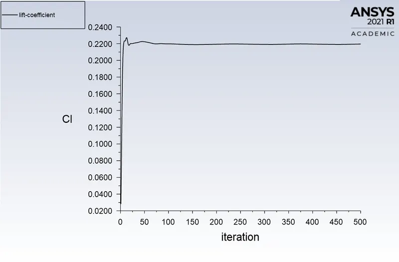
Lift Coefficient Plot

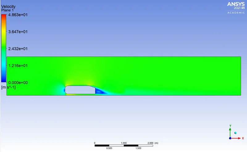
Velocity Contour

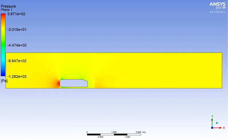
Pressure Contour

Pressure at Car wall

Velocity Vector

Case	Outer Enclosure Mesh size (mm)	Inner Enclosure Mesh size (mm)	Drag Coefficient (Cd)	Lift Coefficient (Cl)
Case 1	100	50	0.3399	0.2075
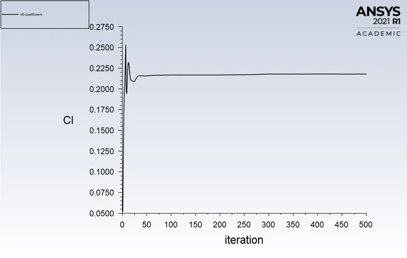
Case 2	100	40	0.3324	0.2178
Case 3	100	35	0.3214	0.2287
Case 4	100	30	0.3092	0.2195

Grid Independence Test:

Case	Outer Enclosure Mesh size(mm)	Inner Enclosure Mesh size (mm)	Number of Elements	Drag Coefficient (Cd)	Lift Coefficient (Cl)
Case 1	100	50	125670	0.3399	0.2075
Case 2	100	40	176863	0.3324	0.2178
Case 3	100	35	225757	0.3214	0.2287
Case 4	100	30	313188	0.3092	0.2195
Case 5	50	40	239250	0.3266	0.2066
Case 6	50	35	298789	0.3188	0.2195
Case 7	50	30	399748	0.3083	0.2358
Case 8	50	27	493704	0.3015	0.2421

Flow Separation and the Significance of the Point of Separation:

Flow separation is the common phenomenon occurring in both external as well as internal flows. The flow separation occurs as air flows around an object such as an aircraft wing, high-rise buildings, vehicles, even around a soccer ball, etc. In wall-bounded internal flows where the fluid flow is expanding along a pipe or when it is taking a `90^0` turn around the corner of an elbow, we see flow separation. The physics responsible for this phenomenon is the same for both internal and external flows.

A thin viscous region called the boundary layer is created when the viscous fluid flows over a stationary solid. In most external flows, the flow outside of this vicious region can be regarded as inviscid. In these boundary layers, the velocity of the fluid at the surface of the object is equal to zero. This is called the no-slip boundary of the fluid. The fluid velocity continues to grow away from the boundary until it nearly becomes equal to the free stream velocity.

For a flow over a horizontal plane, the pressure gradient along the plate is continuously decreasing and remains favorable. Fluid flow can not separate under these conditions and remains attached to the surface. However, for certain boundary layer flows, the fluid encounters adverse pressure gradients, this means the pressure is locally increasing in the direction of flow. Under such conditions, the flow is struggling and the local velocity gradient approaches zero at this point the flow detaches from the surface, and this detachment of fluid flow from the surface is referred to as flow separation. Beyond the separation point, a reverse flow occurs near the surface, and the velocity gradient becomes negative. The streamlines following the surface of the body are now deflected away from the body.

The separation point is defined using a wall shear stress profile along with the flow. Along the surface where the wall shear stress becomes zero is regarded as the point of separation. beyond this point local velocity gets reverse. The wall shear stress changes direction. The relatively low-pressure region behind the body is commonly referred to as wake. Flow separation over a body induces a wake behind the body. the interaction between this forward and reverse flows in the region generates fluid rotation or vortex structure. Depending upon the Reynolds number of the fluid and the shape of the geometry, we can have either laminar or turbulent vortices. The shape of the solid body greatly influences flow separation.

From an engineering perspective in the external flows, flow separation is detrimental to both lift and drag forces. It decreases lift and increases drag.

Streamlining a body helps delay this flow separation and streamlining bodies are employed in most external flows application.

Conditions for boundary layer separation:

	PRESSURE GRADIENT	VELOCITY GRADIENT
NO BOUNDARY LAYER SEPARATION	`(delp)/(delx) <0`	`(delu)/(dely)>0`
POINT OF SEPARATION	`(delp)/(delx) = 0`	`(delu)/(dely) = 0`
BOUNDARY LAYER SEPARATION	`(delp)/(delx) >0`	`(delu)/(dely) <0`

Negative pressure in the wake region:

The separation takes two regions of distribution. One at the upper part of the rear end and the other at the lower part of the rear end. Flow separation over a body induces a wake behind the body. the interaction between this forward and reverse flows in the region generates fluid rotation or vortex structure. Vortex has a strength which we call the circulation that is nothing but vorticity over the area covered by the vortex. So vorticity is continuously generated in the boundary layer and fed into the vortex through the separated shear layer. Once this vortex starts forming, as the vortex has lower pressure in its core so pressure starts falling. The moment pressure reduces it acts as a sink, It will suck flow from all around. Each vortex has lower pressure in its core so when it forms behind the body, the induced pressure field at the rear part of the body will create additional drag because the pressure at the back is less than the pressure in the front. The front has stagnation point highest possible pressure. So there is a drag form by the vortex. So due to the separation of flow, there is emptiness created in the rear end of the body then negative pressure gets developed in the rear portion of the body.