External flow simulation over an Ahmed body.

Aim:- External flow simulation over an Ahmed body in Ansys fluent.

Objectives:-

• To study the Ahmed body as the basis of simulation for external flow over a vehicle.
• To study the evaluation of Y+ value and its importance for simulation.
• To pre-process the geometry and mesh for Ahmed body simulation.
• To refine the mesh and study the effect of coefficient of drag on the Ahmed body.
• To perform the mesh independent test for Ahmed body simulation.

Theory:-

Standard wind tunnel models

Standard wind tunnel models, also known as reference models, calibration models or test check-standards are objects that have relatively simple and precisely defined shapes, that have known aerodynamic characteristics, that are used in wind tunnel tests. Standard models verify, by comparison of wind tunnel test results with previously published results, the complete measurement chain in a wind tunnel, including wind tunnel structure, quality of the airstream, model positioning, transducers and force balances, data acquisition system and data reduction software.

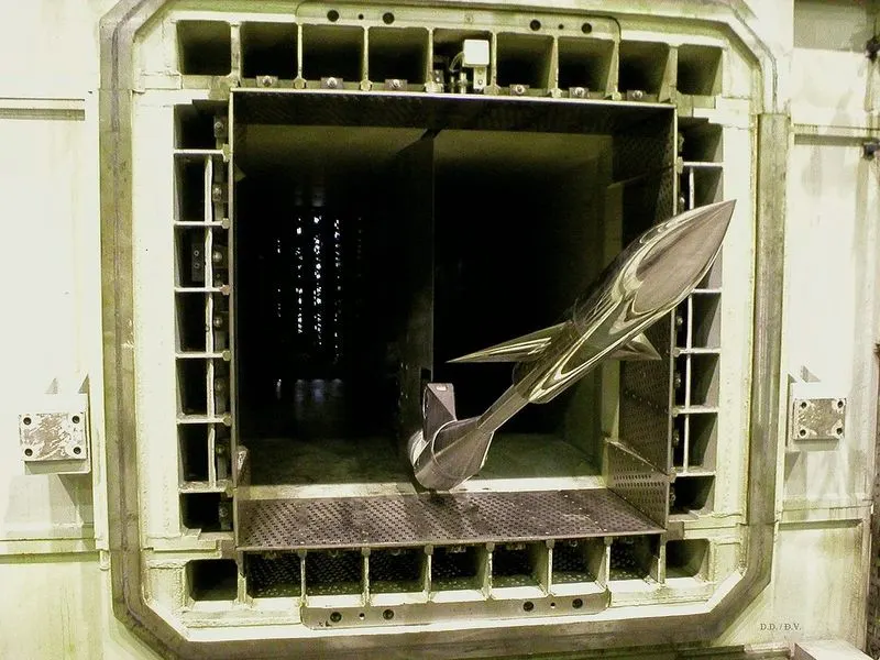
above is, AGARD-B standard wind tunnel model

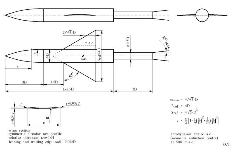
above is the aforementioned model's dimensions, which has known analytical properties.

Standard wind tunnel models are used for:

• To confirm the reliability of the data and to provide baselines for correlation of results from a new wind tunnel by comparing results from other existing wind tunnel facilities.
• checkouts of data repeatability over time and after repairs or modifications of the wind tunnel structure.
• assessment of the wall interference effects.
• Assessment and identification of problems and faults in the operation of a wind tunnel.
• verification of new measurement techniques or devices.
• training of wind tunnel personnel.

Ahmed body model

In the automobile industry, Ahmed Car Body is the standard wind tunnel model that can be used as a validating case, in CFD simulation. Ahmed Body is a generic car-type bluff body with a slant back that has different angles from 0 – 40 degree. Ahmed body is a generic car body (a simplified car model) i.e It is usually used as a benchmark test case for simulating the external aerodynamic flow characteristics over a car model. The flow of air around the Ahmed body captures the essential flow features around an automobile.

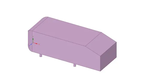
Ahmed body is a simplified car model created by Ahmed et in 1980’s to investigate the behaviour of newly developed turbulence models for complex geometry cases. It’s body is made up of a round front part, a moveable slant plane placed at back part of the body to study the coefficient of drag and separation phenomena at different angles, and a rectangular box, which connects the front part and the rear slant plane. As the wake separation flow behind the Ahmed body is the main contributor to the drag force, accurate prediction of the separation process and the wake flow are the key to the successful modelling of this case.

Ahmed body is a simplified model of a car body, but it demonstrates all the flow features involved in an actual case of a moving car.

Reasons for negative pressure in wake region

Before we discuss why there is a negative pressure region we need to understand the following terms:

1. Wake
2. Flow separation
3. Adverse pressure gradient

Wake

Wake is the region of recirculating flow immediately behind a moving or stationary body, caused by viscosity, which can be accompanied by the separation of flow and turbulence. The boundary layer separation is caused due to adverse pressure gradients, which creates a wake filled with energetic eddies that increases the drag, by dissipating a great deal of mechanical energy.

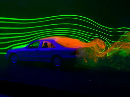
Flow separation and Adverse pressure gradient

Flow separation or boundary layer separation, is the detachment of a boundary layer from a surface to form a wake. After passing the thickest part of a streamline body or passing through a widening passage, separation occurs due to the flow that is slowing down, with pressure increasing. Here the rear part of the Ahmed body that comes after the sloping part is a section that has aggressively widened.

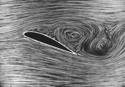
Adverse pressure gradient, is the flow that's flowing against an increasing pressure.This is important for boundary layers. Increasing the fluid pressure means increasing the potential energy of the fluid, which leads to a reduced kinetic energy and a deceleration of the fluid. The slower fluid in the inner part of the boundary layer, is greatly affected by the increasing pressure gradient. This fluid may slow to zero velocity or even become reversed causing a flow separation, if the increase in pressure is large enough. In aerodynamics, since the flow separation significantly modifies the pressure distribution along the surface (and hence the lift and drag characteristics), the consequences are considered to be significant.

Turbulent boundary layers tend to be able to sustain an adverse pressure gradient better than an equivalent laminar boundary layer. The more efficient mixing which occurs in a turbulent boundary layer transports kinetic energy from the edge of the boundary layer to the low momentum flow at the solid surface, often preventing the separation that would occur for a laminar boundary layer under the same conditions. In the automobile industry this physical fact has led to a variety of schemes to actually produce turbulent boundary layers when boundary layer separation is dominant at high Reynolds numbers such as vortex generators and diffusers to improve the areas where point of separation takes place.

When the boundary layer has travelled far enough in an adverse pressure gradient, the speed of the boundary layer relative to the surface stops and reverses direction, causing boundary layer separation. The flow detaches from the surface, and instead takes the forms of eddies and vortices. Once the flow has separated, the fluid exerts a constant pressure on the surface, instead of a continually increasing pressure if the flow would have still been attached.

In aerodynamics, flow separation results in reduced lift and increased pressure drag, caused by the pressure differential between the front and rear surfaces of the object. Much effort and research has gone into the design of aerodynamic and hydrodynamic surface contours and added features which delay flow separation and keep the flow attached for as long as possible. Examples include vortex generators at the roof around c-pillars, on side view mirrors, diffuser below the rear point of the and overall smooth underbelly of the car, and so on.

Negative pressure in wake region

1. Firstly the pressure doesn't increase continually because the flow no longer follows the boundary layer as it separates when the boundary layer has travelled far enough in an adverse pressure gradient. At that point the speed of the boundary layer relative to the surface has stopped and reversed direction. Hence the pressure after the point of separation becomes constant.
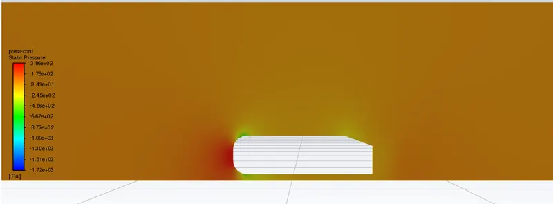
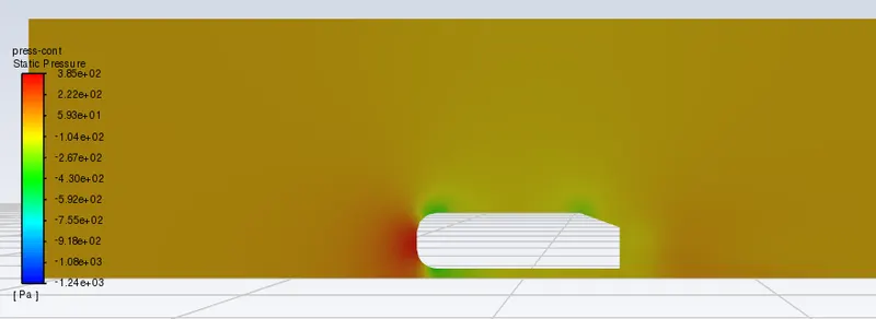
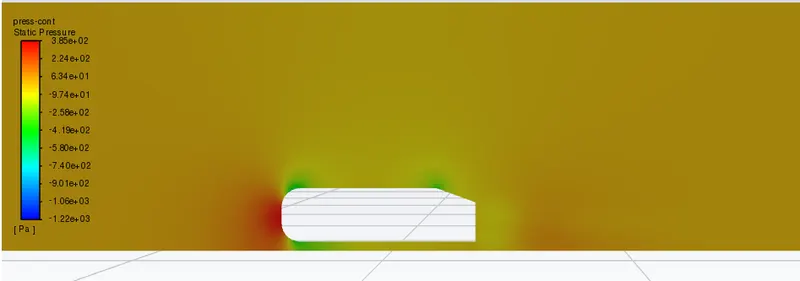
2. And in Ahmed body, when the air hits the frontal face of the body the maximum pressure is created and the flow gets separated into two regions, above the body and below the body. Ahmed body is more of a rectangular shape and hence the separated air along the body travelling to the rear end, doesn't contact the body surface due to wake generation. This causes the void to develop a negative pressure region, where the pressure drops even further at the corners of the Ahmed body which we’ll see in the velocity contours after the simulation has been conducted.

Significance of the point of separation

Flow separation or boundary layer separation, is the detachment of a boundary layer from a surface into a wake.Separation occurs in flow that is slowing down, with pressure increasing, after passing the thickest part of a streamline body or passing through a widening passage. Here the rear part of the Ahmed body that comes after the sloping part is a section that has aggressively widened.

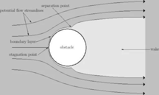
Since the fluid in the inner part of the boundary layer is slower, it is more greatly affected by the increasing pressure gradient. For a large enough pressure increase, this fluid may slow to zero velocity or even become reversed causing a flow separation. This has very significant consequences in aerodynamics since flow separation significantly modifies the pressure distribution along the surface and hence the lift and drag characteristics. Hence the point of separation needs to be optimized to control the drag and lift of the car.

The boundary layer

The boundary layer is a thin layer of a real fluid along the surface of an object in which viscosity affects fluid dynamics. The no-slip condition accounts for zero relative velocity on the surface of an object and keeps on increasing until it reaches the free stream velocity. The shear forces and inertia forces are equally important in determining the motion of the fluid element, within the narrow boundary layer adjacent to the surface and shear stresses can be neglected outside of the region. The thickness of the boundary layer is the distance from the plate until the velocity reaches 99 % of the free stream velocity.

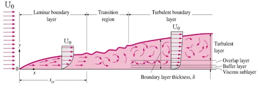
The flow behavior and turbulent structure are considerably different in the presence of the solid boundary when compared to free turbulent flows. Near to the wall the flow is influenced by the viscous effects and independent of free stream parameters. However, the mean flow velocity depends on the distance from the wall(y), fluid density(ρ), viscosity(µ), and wall shear stress(𝛕).

The near-wall results become nonlinear and inconsistent due to the existence of all these layers in the boundary layers. Hence it got very difficult to find the numerical trend line which matches the experimental results. Relationship between velocity and wall distance, was devised In 1905, where Prandtl and his student nikuradse normalized the axes into y+(the axis that is used to be the distance) and u+(the axis that is used to be velocity). They also wrote an equation that would fit u+ and y+ near the wall.

Y plus

Y+ is used to distinguish different regions near the wall or in the viscous region. The size of the mesh should be small and dense enough near the wall so that almost all the effects are captured, If we intend to resolve the effects near the wall i.e., in the viscous sublayer. But in some cases,the coarse mesh would work near the wall if the wall effects are negligible, and if we including semi-empirical formulae to bridge between the viscosity affected region and fully turbulent region.

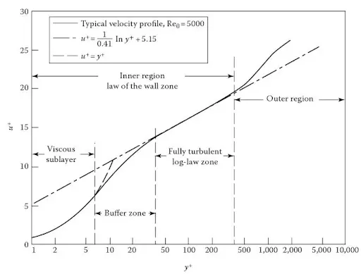
Considering the first case i.e., near-wall modeling it is well-known that the mesh size should be small enough, and based on the y+ value the first cell height can be calculated which decides how small the mesh is going to be exactly. The near-wall region is meshed using the calculated first cell height value with gradual growth in the mesh so that the effects are captured and hence avoiding overall heavy mesh count.

To capture the flow around the Ahmed body it is important to have finer mesh region around the edges. To have better mesh resolution calculation of Y+ value becomes essential to capture the flow near the body. Calculation of Y+ value depends upon free stream velocity and skin friction coefficient of the body. Below is the procedure for calculation of Y+ value and total thickness of the inflation layer:-

Calculations:-

Assumptions and given data:-

Assuming the working fluid is air:-

⍴ = 1.225 kg/m^3

μ = 1.7894e-05 kg/m.s

V = 25 m/s (given)

L = 1.044m (calculated from 3d model)

Assumed Y+ value = 30, since the turbulence model chosen is k-epsilon.

Solution:-

• Reynolds number:-

Re = (ρVL)/μ = 1,786,772

• Skin friction coefficient:-

Cf = (0.026)/(Re)1/7 = 0.003325

• Shear stress near wall:-

𝛕wall = (Cf⋅ρ⋅U2) /2 = 1.2728 N/m^2

• Friction velocity:-

UFric = √((𝛕wall) /ρ) = 1.019

• First layer thickness:-

ΔS = (Y+⋅μ)/(UFric⋅ρ) = 0.001433m

• Total thickness of Inflation for 5 layer:-

TotalThickNess = ΔS⋅((1.2)^5) = 3.56mm

• Total thickness of Inflation for 10 layer:-

TotalThickNess = ΔS⋅((1.2)^10) = 8.87mm

Procedure:-

• Geometry preparation:-

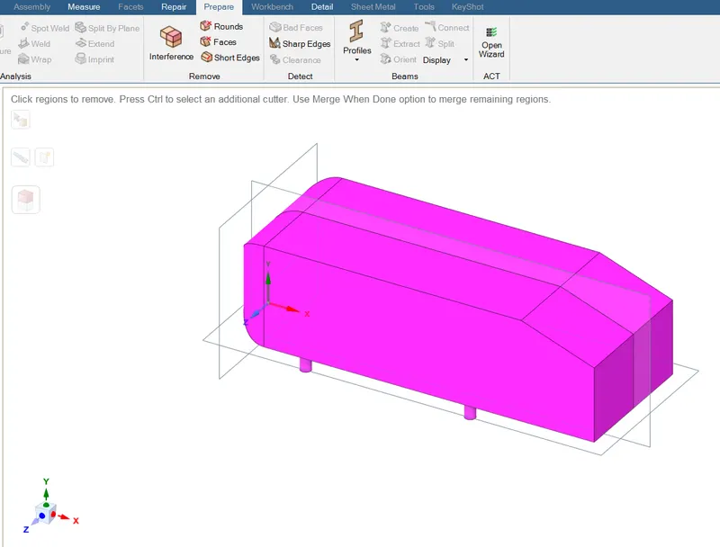
• To split the body in half from the plane of symmetry:- go to design create planes by clicking on origin. Then go to prepare and “select split by plane”, select the body, then select X-Y plane and then choose the side of the body to remove.

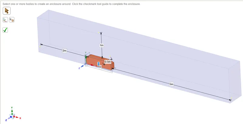
• To prepare an enclosure:- go to prepare, select enclosure, uncheck the symmetric dimension and give the same dimensions as in the following picture(to add another enclosure for the finer meshing follow the same steps but set the dimensions accordingly make sure to fix interference in prepare and choose the share topology option to share from modelling tree)-

• Disable the geometry for physics by selecting the main body from the modelling tree, right clicking and selecting option “diasble for physics”.

• Generating mesh:-

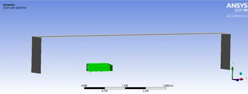
• Creating named selections:- select the nace that needs to be named the press ‘N’ key or right click to select create names selections

• Refining mesh: by adding mesh method, mesh sizing and mesh inflation as well as by refining the Y+ value and total thickness of inflation layer we can get better and more accurate results in the solver.

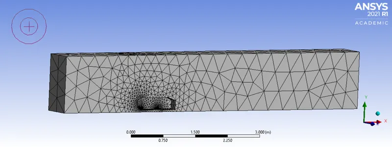
• Check mesh quality in the end, if the quality is above 20% ,your mesh is good for further simulations.

• Setup:-

• Check mesh to ensure there are no quality related issues.
• In general settings, for the type of solver, select ‘pressure-based’ since the mach number is below 0.3 and there are no compressibility effects. And since we only need to find the velocity and pressure distribution and drag force on the body, we can get reliable results with steady state analysis.
• For the turbulence model we use the k-epsilon model,even though it is not the best suitable model for this simulation, but for calculation of Y+ value and since the Reynolds number is quite high, we’ll choose this model.

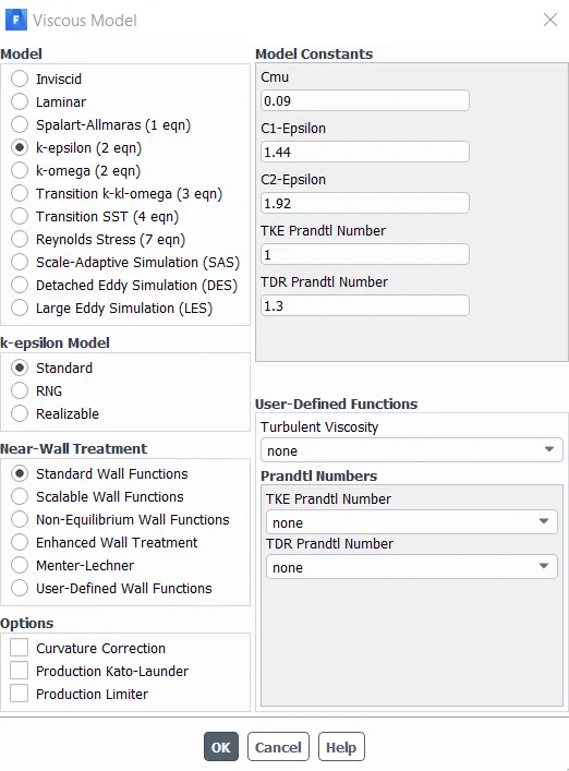
• For material, choose air, which is the default material.
• Then go to set up boundary condition for the case under ‘zones’,there choose ‘inlet’ and set the inlet velocity to 25 m/s. Further check if the ansys has auto-assigned the boundary conditions.

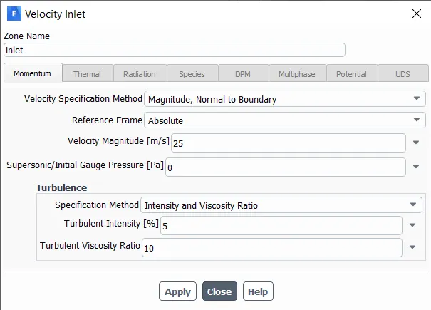
• The the simulation is ready to be solved, go to solution, the check the hybrid method solver then initialize the solution.

• Then go to results, and created an X-Y plane under ‘surface’ and create the plane right in the middle of the body. Then go to contours, create new contour then create velocity and pressure contour on X-Y plane.
• You can also create a solution animation under solution>activities>create>solution animation.

• Result:-

• In the model tree, under the geometry turn on the ‘car-wall’ and under details, colour it by variable>pressure.and apply.
• After that, Insert plane in X-Y plane, same way we made the plane in setup and colour it by velocity.
• To make vector plot,insert>vectors>under ‘location’>select the XY plane that we made.

Observation:-

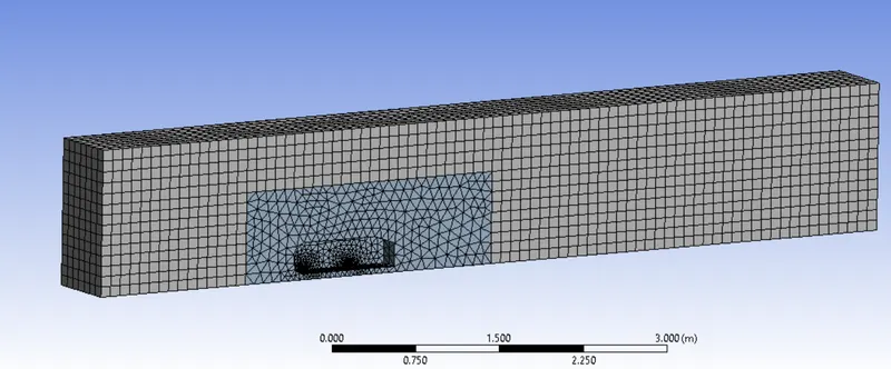
Observations were made based on 4 cases of grid independency tests. the details of the cases are as follows (note:the circular legs of the model are refined separately so that their cross-section dont appear like a polynomial but a circle):-

CASE-1: Flow simulation with default mesh setup.

CASE-2: Flow simulation with 0.1m mesh size for all bodies.

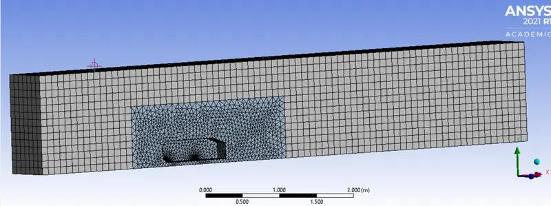
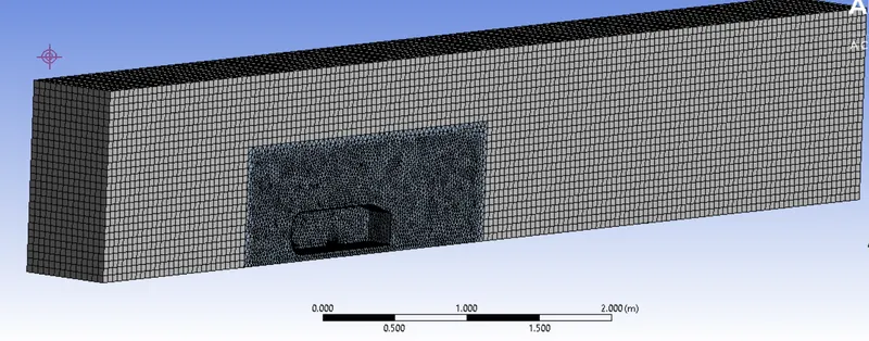
CASE-3: Flow simulation with 0.1m for outside enclosure and 0.05m for inside enclosure with 5 inflation layers.

CASE-4: Flow simulation with 0.1m mesh size for outside enclosure and 0.0243m mesh size for inside enclosure with 10 inflation layer(maximum cell count).

CASE-1:

NUMBER OF ELEMENTS = 42,770

RESIDUALS:

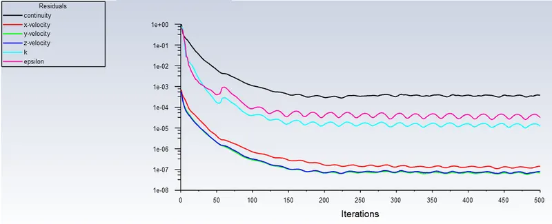
VELOCITY CONTOUR:

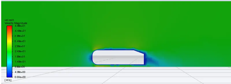
PRESSURE CONTOUR:

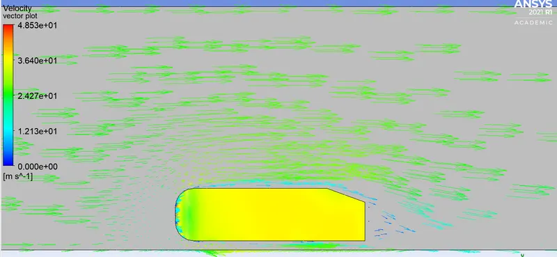
VELOCITY VECTOR:

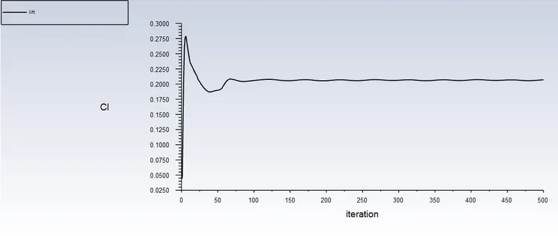
LIFT COEFFICIENT:

Cl=0.206

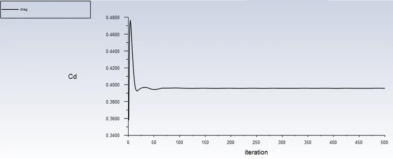
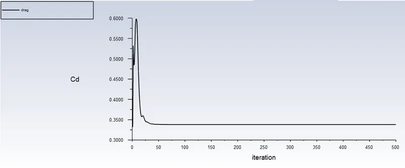
DRAG COEFFICIENT:

Cd=0.395

CASE-2:

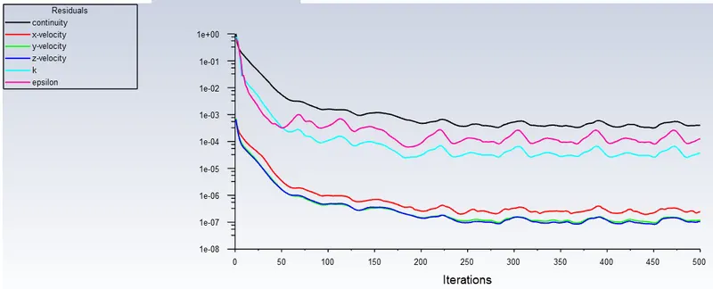
NUMBER OF ELEMENTS = 50399

RESIDUALS:

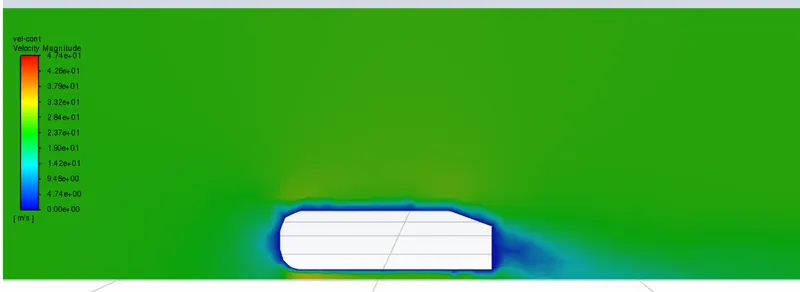
VELOCITY CONTOUR:

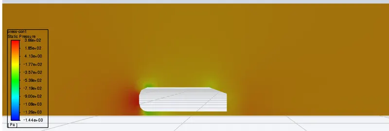
PRESSURE CONTOUR:

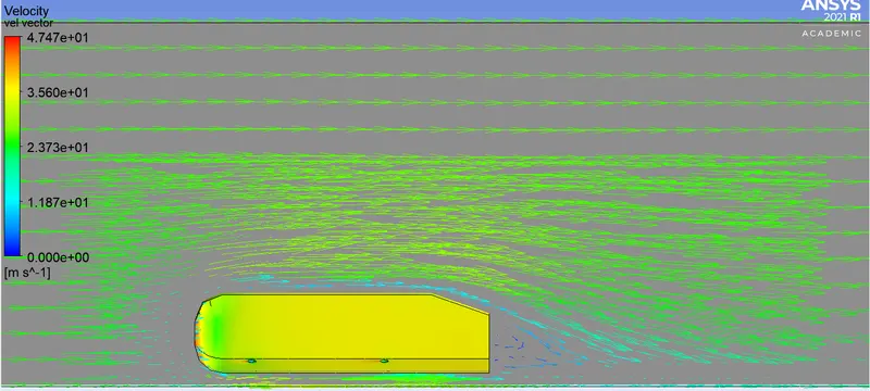
VELOCITY VECTOR:

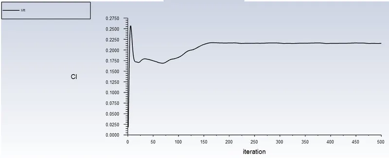
LIFT COEFFICIENT:

Cl=0.21

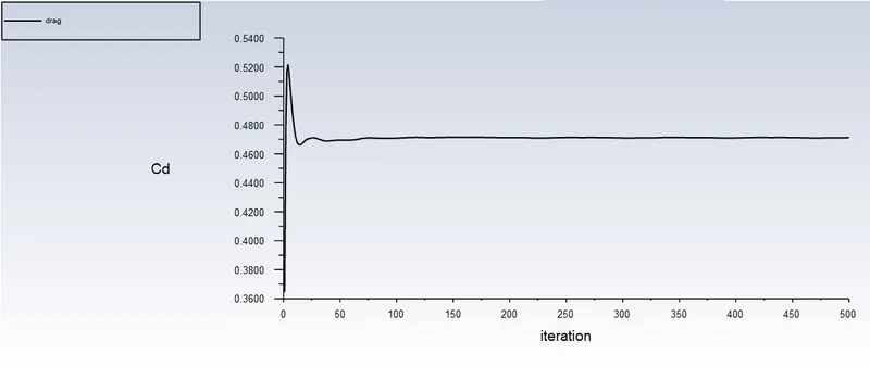
DRAG COEFFICIENT:

Cd=0.47

CASE-3:

NUMBER OF ELEMENTS=1,04,383

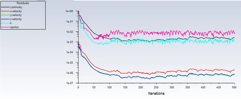
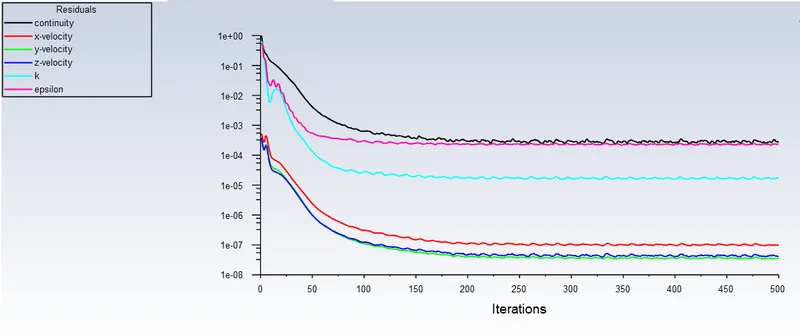
RESIDUALS:

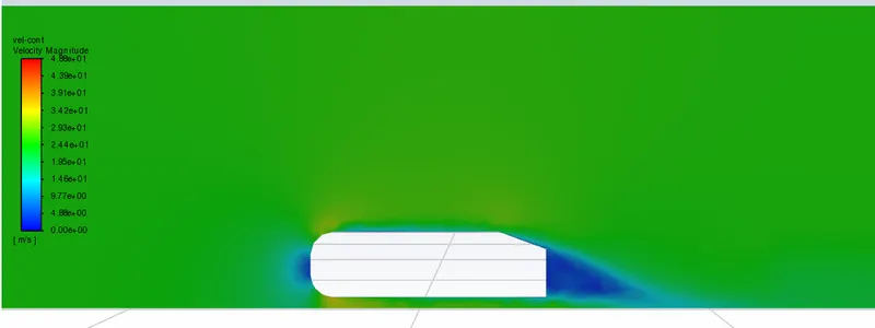
VELOCITY CONTOUR:

PRESSURE CONTOUR:

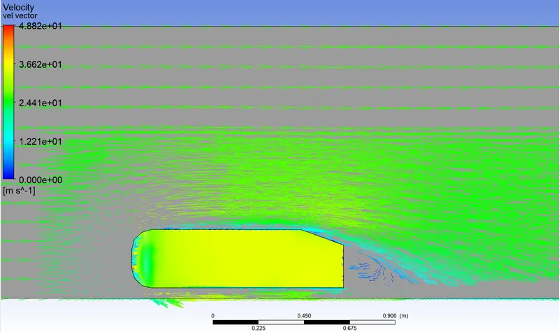
VELOCITY VECTOR:

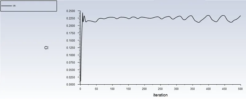
LIFT COEFFICIENT:

Cl=0.23

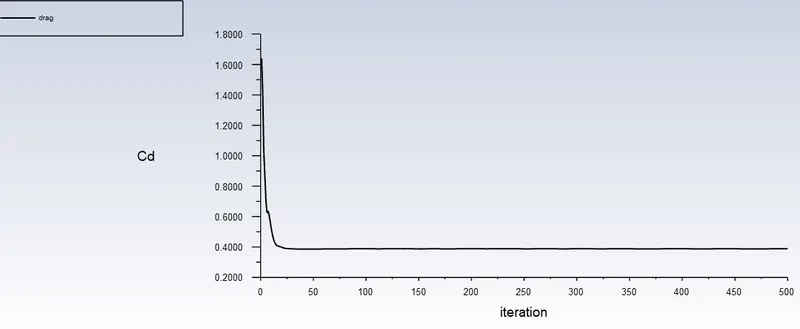
DRAG COEFFICIENT:

Cd=0.38

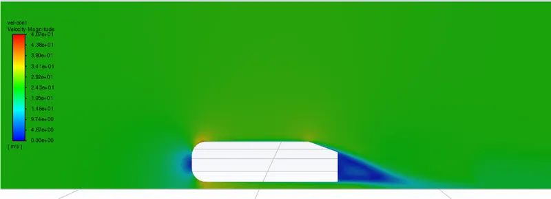
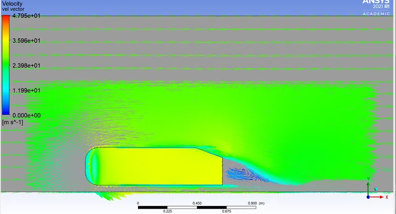
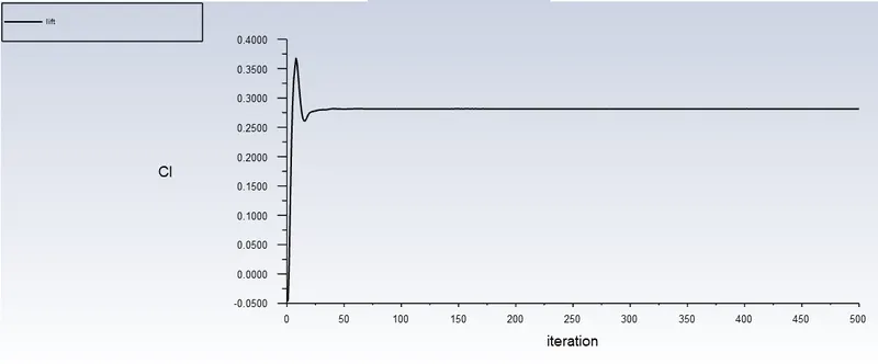
CASE-4:

NUMBER OF ELEMENTS=4,99,376 (maximum possible size)

RESIDUALS:

VELOCITY CONTOUR:

PRESSURE CONTOUR:

VELOCITY VECTOR:

LIFT COEFFICIENT:

Cl=0.28

DRAG COEFFICIENT:

Cd=0.33

Inference:-

• By simulating each case, we found that as the mesh got finer, the result kept getting nearer to accuracy. Also the coefficient of drag decreases and coefficient of lift increases in value.
• Case 4 provide results closest to accuracy benchmark(i.e. value of Cd=0.33) in the wake region when compared with the rest of the cases due to better mesh resolution near the boundary of Ahmed body.
• The velocity before the body is higher as compared to the region behind the body because of wake generation. Similarly, we can see the pressure gradient throughout the flow field.
• The cause of flow separation in the fluid flow is because of negative pressure generation in the boundary layer of flow near the wall of body and negative wake region is generated due to the pressure difference between low stream and high stream flow also due to flow separations. This happens in Ahmed body due to the aggressive widening of the passage at the rear.

Conclusion:-

• Successfully conducted external flow simulation over an Ahmed body.
• Described and calculated Y+ value in the appropriate range to get correct value for drag coefficient.
• Described Ahmed body and its importance.
• Explained the reason for the negative pressure in the wake region.
• Explained the significance of the point of separation.
• Performed the grid independency test and provided the values of drag and lift with each case.
• Made the vector plot, velocity and pressure contours, clearly showing the wake region.