Aerodynamic flow simulation over an Ahmed body

I. Aim: Aerodynamic flow simulation around an Ahmed body using Ansys fluent.

II. Introduction:

The Ahmed body is a generic car body (a simplified vehicle model). The flow of air around the Ahmed body captures the essential flow features around an automobile and was first defined and characterized by Ahmed [1] in his experimental work. Ahmed body is of a simple shape, which allows us to capture characteristic features that are relevant to bodies in the automobile industry.

The Ahmed body is a benchmark model widely used in the automotive industry for validating simulation tools because complexly shaped cars are very challenging to model and it’s difficult to quantify the aerodynamic drag computationally.

The simple geometrical shape of the Ahmed body has a length of 1.044 meters, a height of 0.288 meters, and a width of 0.389 meters. It also has 0.05-meter cylindrical legs attached to the bottom of the body and the rear surface has a slant that falls off at angles in the range of 25-40 degrees. The geometry used by Ahmed in his work is shown below:

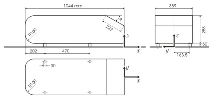
Figure 1: Dimensions of the Ahmed Body (`phi` = 25 degress) [1].

Drag coefficient in cars:

The resistance experienced by a fluid environment to an object in motion is quantified in terms of drag force. Generally, the forces acting on an object in motion or a stationary object in a flowing fluid are classified into drag and lift forces. The component parallel to the fluid flow direction is called the drag force and the forces perpendicular to the fluid flow direction are called lift forces.

The drag force acting on a body is given by the formula:

`F_d = 1/2C_drhoAV^2` .

where, `F_d` = Drag force in Newtons

`C_d` = drag coefficient

`rho` = Density of the fluid in kg/m^3

A = frontal area of the object in m^2

V = fluid velocity/object velocity in m/s.

The lift force acting on a body is given by the formula:

`F_l = 1/2C_lrhoAV^2`

where, `F_l` = lift force in Newtons

`C_l` = lift coefficient

`rho` = Density of the fluid in kg/m^3

A = frontal area of the object in m^2

V = fluid velocity/object velocity in m/s.

Generally, ground vehicles(ex: cars) experience lift forces rarely while in motion, hence the study of drag forces on automobiles is important. The drag coefficient is a nondimensional way of expressing drag force, and it varies for different objects and also depends on the flow Reynolds number.

The lower the drag coefficient of an object, the less aerodynamic or hydrodynamic drag occurs. In terms of a car, the lower the drag coefficient, the more efficient the car is. As well as affecting the top speed of a vehicle, the drag coefficient also affects the handling. Cars with a low drag coefficient are sought after, but decreasing the drag drastically can reduce the downforce and lead to a loss in road traction and a higher chance of car accidents. The drag coefficient value ranges from 0.3-0.35 in most commercial cars. The value may be higher in SUVs and will be lesser than 0.3 in streamlined cars[3].

In this project, the numerical analysis of flow around the Ahmed body is carried to validate the numerical model using the commercial CFD simulation tool Ansys Fluent.

III. Objectives:

1. To simulate the aerodynamic flow around an Ahmed body in Ansys Fluent

2. Calculate the drag coefficient on the Ahmed body for a flow velocity of 25 m/sec.

3. Perform grid independence study and calculate the lift and drag forces.

IV: Solving & Modelling approach:

3D CFD analysis is carried out in Ansys workbench using Fluent solver to simulate the flow around the Ahmed body for a wind flow velocity of 25 m/s.

V: Pre-processing and solver setting:

The first step in a CFD analysis is preprocessing. This includes preparing the geometry/ computational domain, discretization of the domain (meshing), assigning material properties, boundary conditions, solver setup.

1. Geometry/Domain:

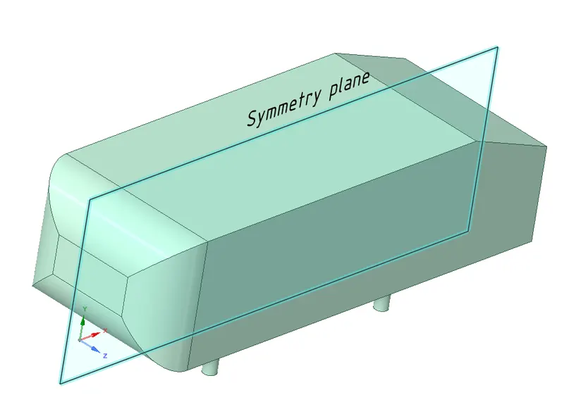
The 3D computational domain is prepared using Ansys space-claim design modeler. Since the Ahmed body and the flow are symmetric along the length direction, only half of the Ahmed body is considered with the central plane of the Ahmed body acting as a symmetric plane. The Ahmed body considered for the analysis has a rear slant angle `phi` = 20 degrees. The fluid domain is generated by enclosing the Ahmed body with enclosures around it. Two enclosures are created with shared topology enabled between them. The inner enclosure is created to have a refined mesh surrounding Ahmed body. The details about geometry and fluid domain are given in the below figures:

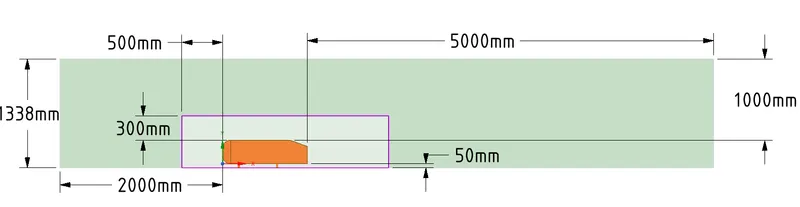Figure: Isometric view of the Ahmed body with symmetry plane	Figure: Ahmed body enclosed in the fluid domain with enclosure dimensions (Symmetry plane view)

2. Domain discretization /Meshing:

The 3d fluid domain is discretized into a finite number of control volumes using the Ansys meshing component. A 3D all hexahedral mesh is created for the outer fluid domain using the multizone meshing method and all triangular mesh for the inner domain surrounding the Ahmed body to accurately capture the geometry. The cells near to the Ahmed body outer surfaces are inflated using the global inflation option to create boundary layer cells. A total of 10 boundary layer cells are created with a first-layer thickness depending on a y+ value and a growth rate of 1.2. A totla of 6 different mesh combinations are used with different y+ values and inner domain mesh refinements. The section view of generated 3D mesh for the case of y+ = 50 with a cell count of 209115 is shown below:

y+ value:

In order to capture the wall-bounded turbulence effect, the cells near the wall should be inflated and the nondimensional first cell height y+ value determines how effectively the physics is captured. In this analysis, the flow Reynolds number (Re ) is around 1.78E6 (> 5E5). Hence the flow is turbulent in nature. The `k-epsilon`model with standard wall function is used in this analysis since the flow has no separation effects. For this model to be used the value of y+ should be in the range of 30 to 300. The first cell height calculated from the following relations :

`y+ = (y*rho.U_tau)/nu`

where y = height of first cell centroid in the mesh

`U_tau = sqrt(tau_w/rho)` is the friction velocity at wall

The shear stress `tau_w`is calculated using the empirical formula

`tau_w = 1/2 C_f*rhoV^2`

`C_f = 0.058Re^-0.2` , for flow over a flat plate

From the above relations and choosing a suitable value of y+, the y value can be determined. The height o the first cell is 2 times of y.

The fluid considered for the analysis is air at atmospheric conditions. The flow conditions are given in the below table:

Flow conditions
Fluid	Density (kg/m^3)	Dynamic viscosity (Pa.s)	Flow velocity (m/s)	Reynolds number (Re)
Air at atmospheric conditions	1.225	1.789E-5	25 m/sec	1.78E6

Considering the above flow conditions, the following y+ values are used for the analysis and the corresponding first cell height are given below:

y+ value	y (m)	First cell height (m)
50	7.24E-4	1.447E-3
35	5.07E-4	1.01E-3
30	4.34E-4	8.69E-4

The boundaries of the domain are also defined in the Ansys mesher using the named selection option. The boundaries are defined as follows:

Boundary/Zone	Boundary/Zone name
Inlet	inlet
Outlet	outlet
Ahmed body walls	Ahmed body
Symmetry plane	symmetry_plane
Side,bottom,Top walls	symmetry

3. Solver setup:

The 3D analysis is performed on the discretized domain(meshed model) in Ansys Fluent CFD software. A double-precision parallel solver with 4 cores is used. The double-precision solver uses 64-bit precision, which reduces the round-off error in the results.

The pressure-based solver is considered for the analysis. The steady-state analysis is considered as the solution parameters of interest ae drag and lift forces, which can be obtained from a steady-state solution.

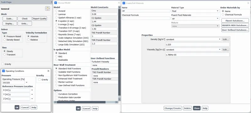
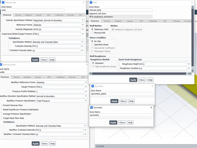
The type of solver, operating conditions, viscous model, material properties, zones, and boundary conditions are defined in the respective section of the physics tab as in the below figures. The operating conditions define the atmosphere in which the analysis is carried out. This sets the reference pressure. In this analysis, a reference pressure of 1 Bar(101325 Pa) is considered to simulate atmospheric conditions. The `k-epsilon` model with the standard wall functions option is selected in the viscous option of the models section. The default air in the fluent database is used as the fluid material. Cell zones are defined to apply the materials to the domains. In the current problem, we have only one zone ie. fluid zone with material as 'air'.

The inlet velocity is defined as 25 m/sec. The outlet BC is a pressure type with gauze pressure equal to zero, as it is open to the operating condition(atmosphere).

These along with wall boundary conditions of no-slip for Ahmed body and symmetry BC are assigned in the boundaries option of the zones section.

The below images represent the BC assignment in Fluent.

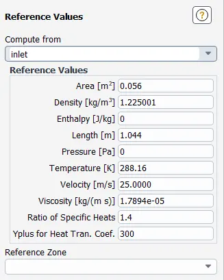
Reference Values:

In order to calculate the drag and lift forces on the cylinder, the reference frontal area of the Ahmed body facing the air flow direction along with fluid flow properties are defined in the reference values section as shown below:

Solution setup:

After setting up the operating conditions, material properties, zones, and boundary conditions, the solution method, controls, type of reports required, initialization type, and a number of iterations to solve are defined in the solution tab.

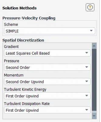
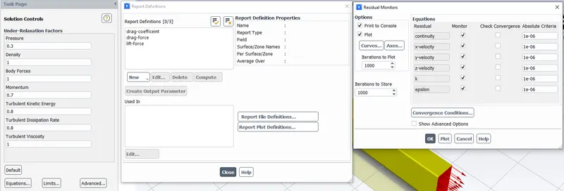
The default simple algorithm is used for the analysis. The simple algorithm solves the momentum and continuity equation sequentially to compute velocity and pressure in the flow field. The discretization schemes chosen for flow variables and gradients are as shown below. The under-relaxation factors for better convergence are also defined in control methods. The reports of drag coefficient, drag force, and lift forces are defined in the reports tab and drag coefficient is plotted to monitor them during the solution. The convergence criteria for the governing equations can be set up using residual monitors in the report section.

VI. Solution Initialization and Run:

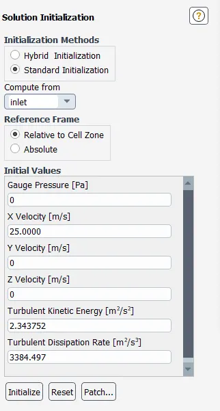
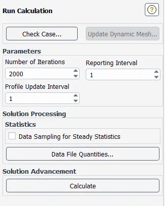
After setting all the above setup conditions, initialization of the domain has to be done necessary, because the solution is an iterative process that can only be executed if there is an initial guess of the solution variables. standard initialization is employed in the current project, computing the initial values in the domain from the inlet . The solution is run iteratively with parameters as given below:

VII. Results and Discussion:

After the solution process is completed, post-processing has to be done to extract and analyze the results. Post-processing is done in Fluent as well as Ansys dedicated postprocessor CFD-Post.

Case 1: y+ value of 50 and mesh count of 209115 cells

Convergence plots:

Residuals	Drag coefficient , Cd on the Ahmed body

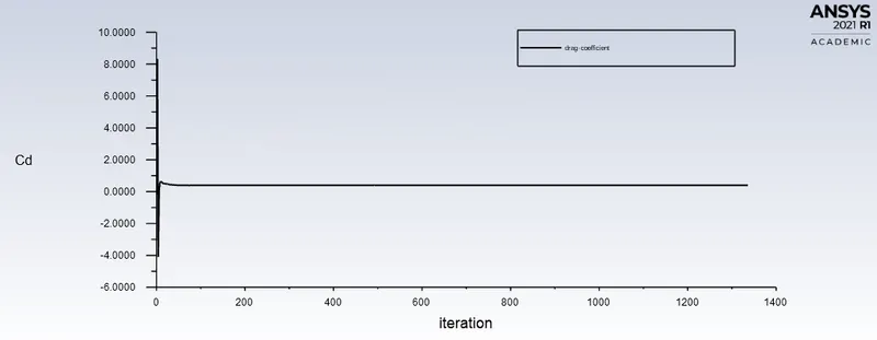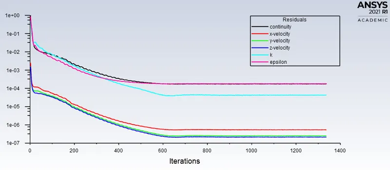
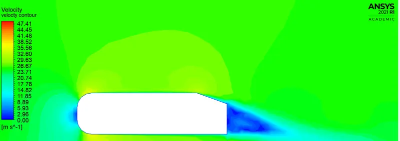
It can be seen from the above plots, that the residuals, drag coefficient (Cd), become constant from around 700 iterations. Hence the solution is said to be converged after 700 iterations.

Velocity contour :	Velocity vectors

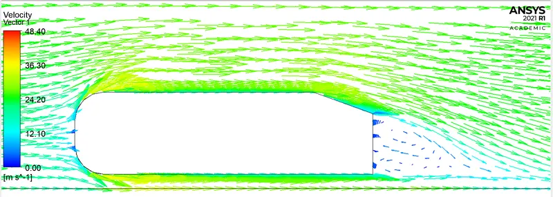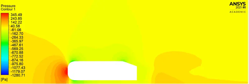
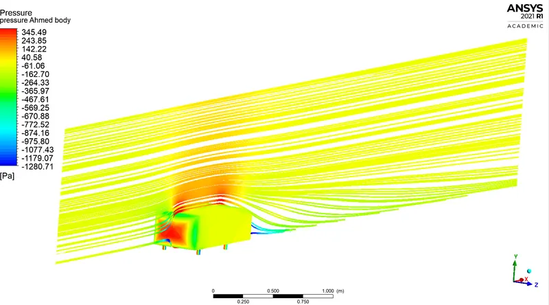
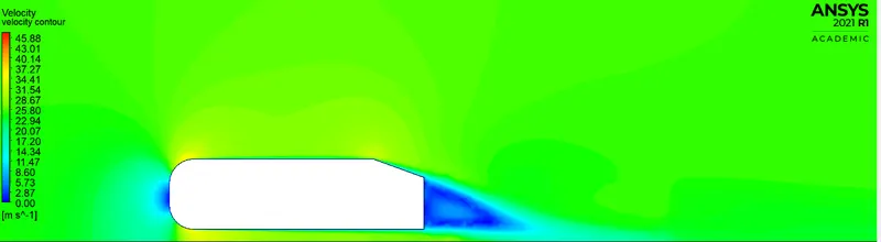
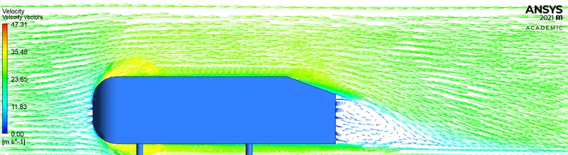
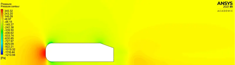
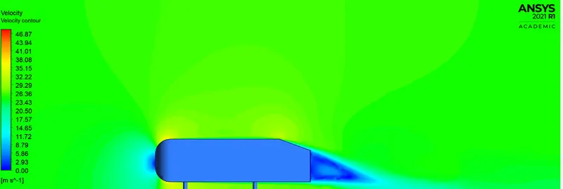
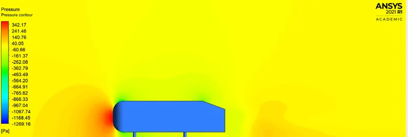
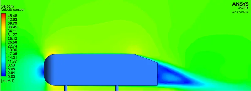
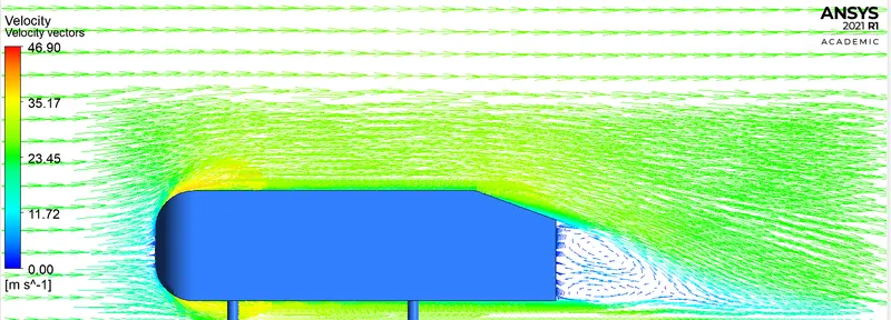
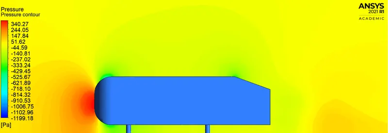
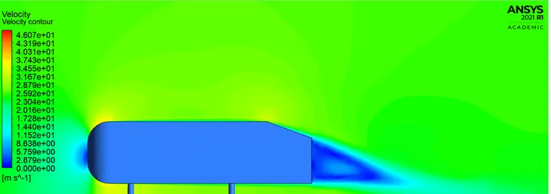
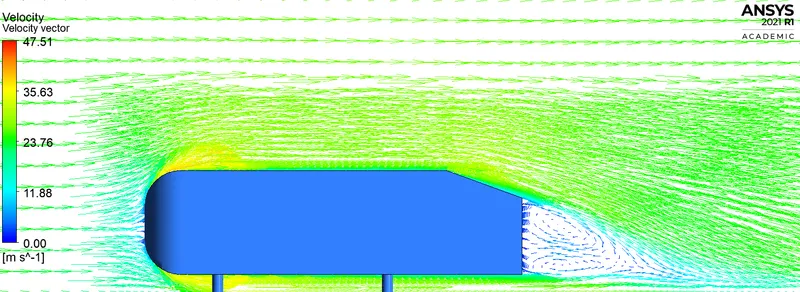
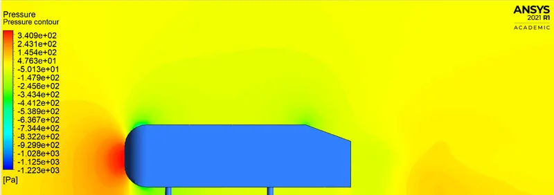
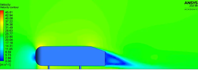
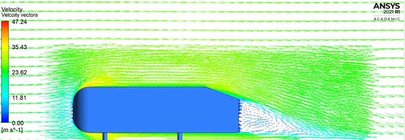
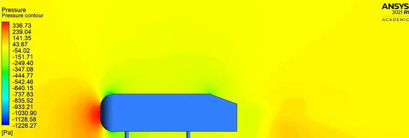
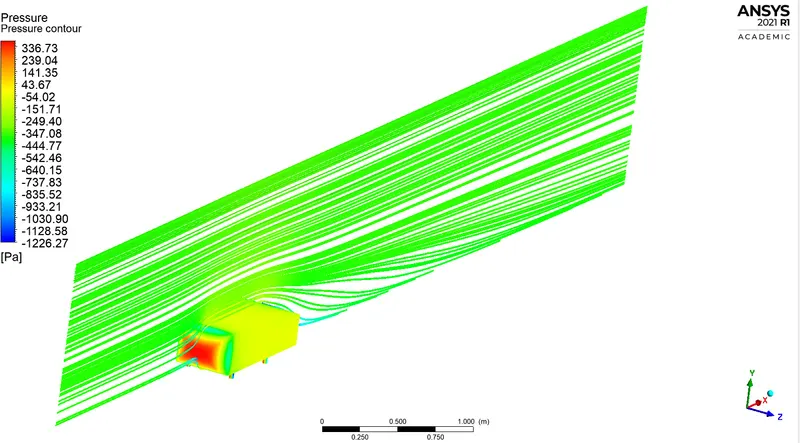
The above plots (Contour and vector) the velocity magnitude distribution around the Ahmed body on passing through the midsection of Ahmed body. It can be seen that the flow attains a stagnation point at the front of the Ahmed body and the flow separates over it. At the rear end of the Ahmed body, the boundary layers detach from the surface and combine far from the body. Since the body is of a bluff nature, there exists a region of considerable size behind them where the flow is slowed down. This region is termed the wake (blue region behind the body). The separation of flow leads huge pressure gradient between the front and rear of the body. There exists a high-pressure region or stagnation point on the forebody and then the pressure drops around the body. Very low pressure (well below free stream value) dominates the wake region. This leads to negative pressures in the wake region as shown in the below pressure contour plots leading to an increase in the drag experienced by the body. Also, due to adverse pressure gradient in the wake, the flow reversal occurs in the wake region leading to the formation of eddies as shown in the above velocity vector plots. The drag coefficient Cd is found to be 0.394.

Pressure contour :	Pressure distribution on the Ahmed body along with flow streamlines at the midsection

Case 2: y+ value of 50 and mesh count of 393038 cells

In this case, the mesh is refined in the region around the Ahmed body to a higher cell count than Case1.

Convergence plots:

Residuals	Drag coefficient , Cd on the Ahmed body

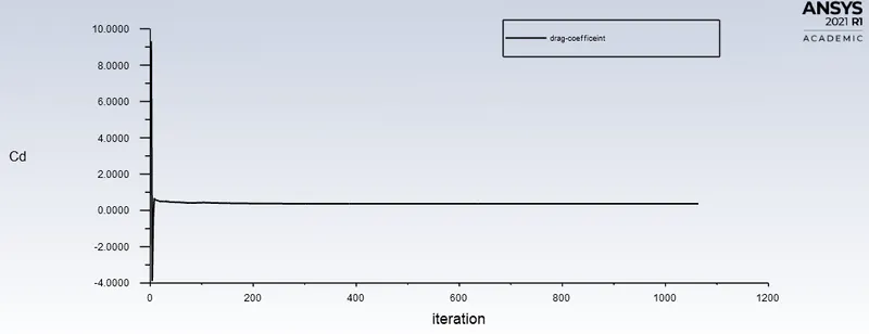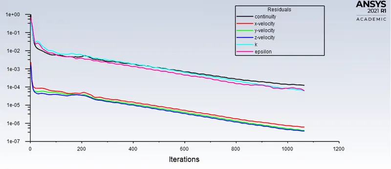
It can be seen from the above plots, that the residuals fall below acceptable limits and the drag coefficient (Cd), becomes constant from around 1000 iterations.

Hence the solution is said to be converged after 1000 iterations. The following plots show the velocity and pressure distribution around the Ahmed body.

Velocity contour :	Velocity vectors

Pressure contour :	Pressure distribution on the Ahmed body along with flow streamlines at the midsection

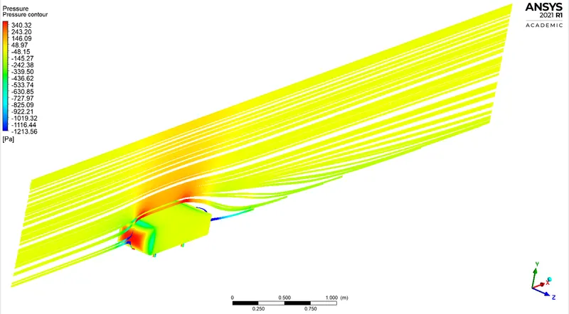The flow dynamics are similar to that of case 1. The drag coefficient Cd in this case is found to be 0.365.

Case 3: y+ value of 35 and mesh count of 398131 cells

In this case, the mesh is refined in the region around the Ahmed body to a higher cell count than Case2, and the y+ decreased to 35.

Convergence plots:

Residuals	Drag coefficient , Cd on the Ahmed body

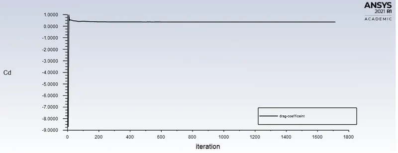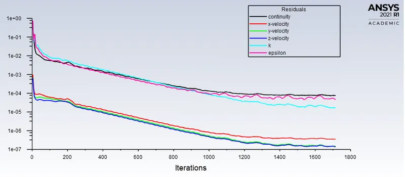
It can be seen from the above plots, that the residuals fall below acceptable limits and the drag coefficient (Cd), becomes constant from around 1400 iterations.

Hence the solution is said to be converged after 1400 iterations. The following plots show the velocity and pressure distribution around the Ahmed body.

Velocity contour :	Velocity vectors

Pressure contour :	Pressure distribution on the Ahmed body along with flow streamlines at the midsection

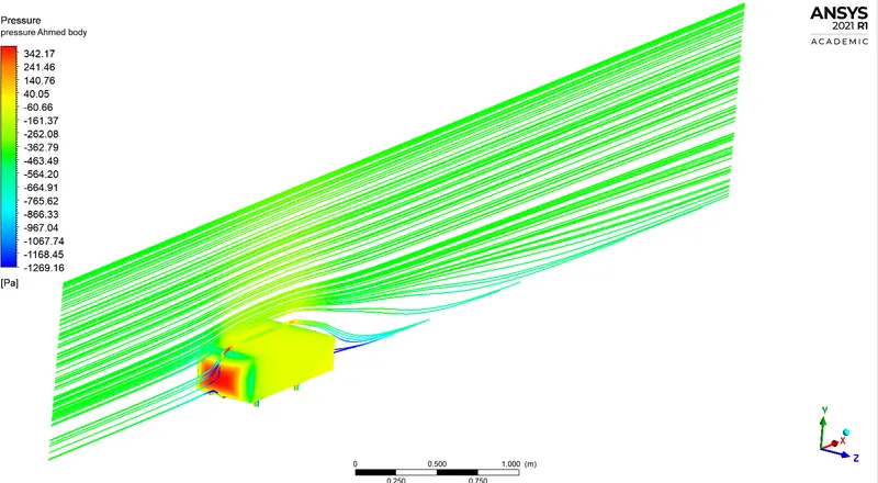The flow dynamics are similar to that of case 3. The drag coefficient Cd in this case is found to be 0.363.

Case 4: y+ value of 35 and mesh count of 447175 cells

In this case, the mesh is refined in the region around the Ahmed body to a higher cell count than Case3.

Convergence plots:

Residuals	Drag coefficient , Cd on the Ahmed body

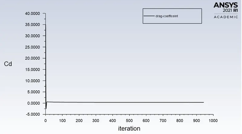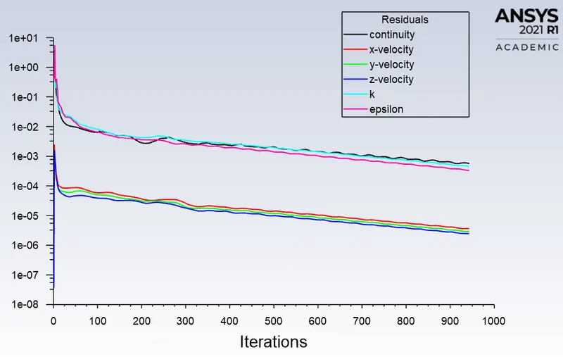
It can be seen from the above plots, that the residuals fall below acceptable limits and the drag coefficient (Cd), becomes constant from around 900 iterations.

Hence the solution is said to be converged after 900 iterations. The following plots show the velocity and pressure distribution around the Ahmed body.

Velocity contour :	Velocity vectors

Pressure contour :	Pressure distribution on the Ahmed body along with flow streamlines at the midsection

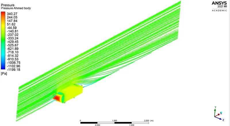The flow dynamics are similar to that of case 2. The drag coefficient Cd in this case is found to be 0.352.

Case 5: y+ value of 30 and mesh count of 450443 cells

In this case, the mesh is refined in the region around the Ahmed body to a higher cell count than Case4 and y+ decreased to 30.

Convergence plots:

Residuals	Drag coefficient , Cd on the Ahmed body

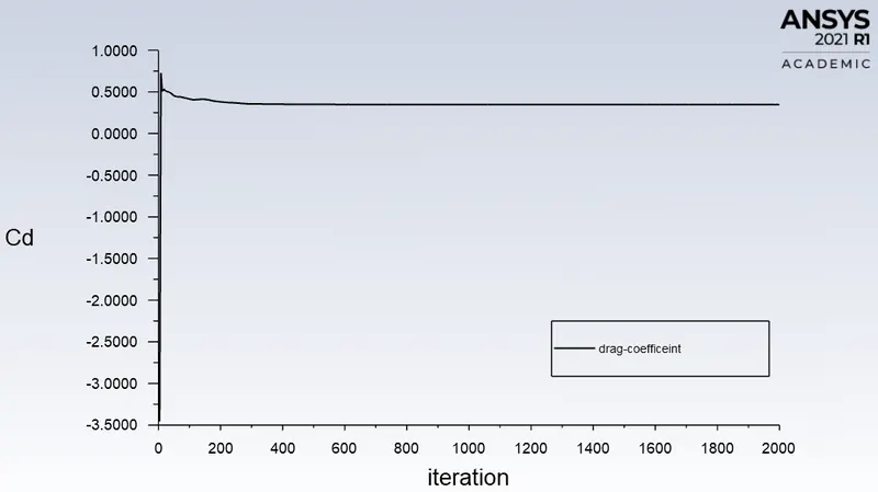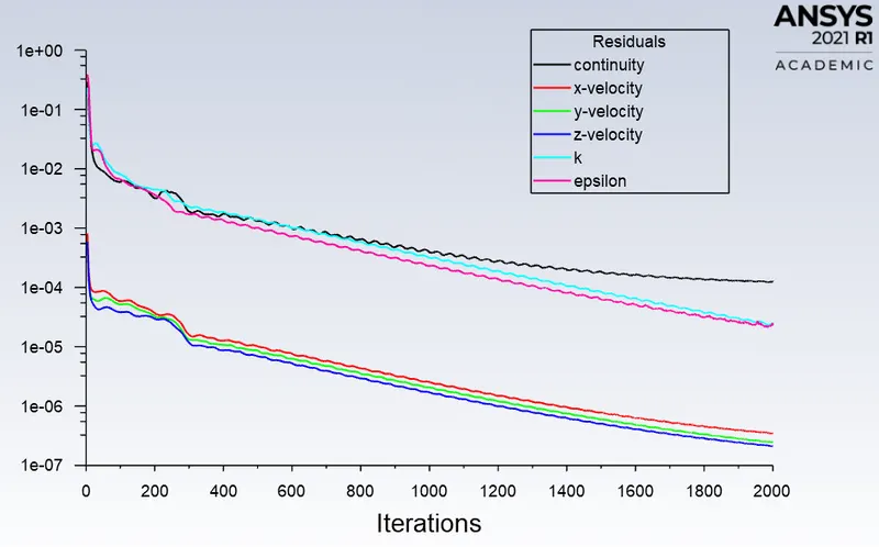
It can be seen from the above plots, that the residuals fall below acceptable limits and the drag coefficient (Cd), becomes constant from around 1600 iterations.

Hence the solution is said to be converged after 1600 iterations. The following plots show the velocity and pressure distribution around the Ahmed body.

Velocity contour :	Velocity vectors

Pressure contour :	Pressure distribution on the Ahmed body along with flow streamlines at the midsection

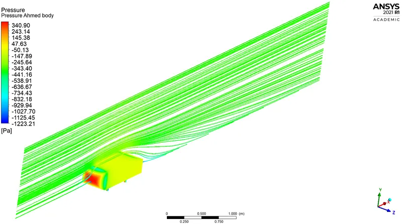The flow dynamics are similar to that of case 4. The drag coefficient Cd in this case is found to be 0.347.

Case 6: y+ value of 30 and mesh count of 479855 cells

In this case, the mesh is refined in the region around the Ahmed body to a higher cell count than Case5.

Convergence plots:

Residuals	Drag coefficient , Cd on the Ahmed body

It can be seen from the above plots, that the residuals fall below acceptable limits and the drag coefficient (Cd), becomes constant from around 1600 iterations.

Hence the solution is said to be converged after 1600 iterations. The following plots show the velocity and pressure distribution around the Ahmed body.

Velocity contour :	Velocity vectors

Pressure contour :	Pressure distribution on the Ahmed body along with flow streamlines at the midsection

The flow dynamics are similar to that of case 4. The drag coefficient Cd in this case is found to be 0.344.

Grid Independence and results comparison:

The following table compares the grid independence and comparison of numerical results with respect to y+ plus value.

Case	Mesh count	Mesh Quality	y+	first cell height (m)	`C_d`	Drag force , `F_d` (N)	Lift force , `F_l` (N)
1	209115	0.68	50	1.45E-03	0.392	8.418 N	6.88
2	393038	0.78	50	1.45E-03	0.365	7.84	6.29
3	398131	0.78	35	1.01E-03	0.363	7.78	6.41
4	447175	0.77	35	1.01E-03	0.350	7.5	6.32
5	450443	0.76	30	8.69E-04	0.347	7.45	6.22
6	479855	0.75	30	8.69E-04	0.344	7.37	6.71

From the above table, it can be inferred that the Cd value doesn't vary much in case 6 when compared to case5. Hence the solution is grid-independent at case 6 with a y+ value of 30 and mesh cell count of 479855 cells. The drag coefficient is 0.344. This value is similar to that of found in the literature [1],[4],[5].

Conclusion:

In this project 3D, aerodynamic flow around an Ahmed body is studied using the Ansys Fluent software. Since it is a bluff body, wake forms at the rear side leading increase in drag. Formation of eddied due to flow reversal as an effect of the adverse pressure gradient is observed. The value of the drag coefficient is found to be influenced highly by the y+ value. Hence choosing the correct y+ value is important while capturing the boundary layer physics around the Ahmed body. The Cd value of 0.344 for a y+ 30 is obtained from the numerical analysis. This value is similar to the values obtained by other researchers.

References

1. Ahmed, S., Ramm, G., and Faltin, G., "Some Salient Features Of The Time-Averaged Ground Vehicle Wake," SAE Technical Paper 840300, 1984.

2. https://www.simscale.com/docs/validation-cases/aerodynamics-flow-around-the-ahmed-body/

3. https://www.comsol.com/blogs/studying-the-airflow-over-a-car-using-an-ahmed-body/

4. Flow and Turbulence Structures in the Wake of a Simplified Car Model (Ahmed Modell)

5. Experiments and numerical simulations on the aerodynamics of the Ahmed body