Week 3 - External flow simulation over an Ahmed body.
Aim:
To understand the drag and lift phenomenon on an ahmed body by flowing air over it at a velocity of 25 m/s.
To find the velocity and pressure distribution around the ahmed body at that particular free stream air velocity.
To check if there is any wake region formed behind the ahmed body.
Introduction & Theory:
Understanding the fluid flow over a solid body is very important in engineering as this can be seen in this almost all engineering applications.
How the flow of fluid is effected when it comes in contact with any solid structure should be understood by solving a wide range of engineering problems.
One of the application of fluid structure interaction is aerodynamics of automobiles and aircraft. Drag and lift are two major forces acting on an automobile/aircraft when in motion. The magnitude of these forces primarily depends on the geometry of the automobile/aircraft.
In case of automobiles, the external curvature on which air flow is responsible for the drag and lift forces. As discussed in the previous problem, when fluid flows over any solid structure, a wake region is formed behind the body and vortices are created. If the frequency of vortices matches with natural frequency of solid body, it would induce vibrations in the solid body and eventually the body will fail.
A wake is a region of disturbed flow behind the solid body . This is a region of low pressure and high turbulence. Flow recirculation might happen here and due to this, vortices are created.
This wake region appears because of flow separation. Because of the curvature of solid body , fluid gets separated and a low pressure region is formed. Understanding how and when wake is created is very important in the design of structures.
As said above, in case of automobiles, wake can form behind if the flow gets separated. This behaviour needs to separated. This behaviour needs to be studied to design automobile structures.
One such study can be done on a solid body called "Ahmed Body".
Ahmed body is a simplified car body. Fluid is flown around this body and essential flow features like drag, lift, velocity, pressure and wake formation can be obtained. Flow velocity can be varied to understand how the above mentioned essential features change. This Ahmed Body allows engineers to capture characteristic features which are relevant to solid bodies in automobile industry. It is used as a test case for evaluating accuracy of numerical simulations in predicting aerodynamic forces and flow separation.
By simulating fluid flow around this body, aerodynamic performance of vehicles can be analysed and thereby designs can be optimized to reduce drag and improve fuel efficiency.
Solving and Modelling Approach:
Whenever fluid flows over a solid body or when a moving body flows through a fluid, the fluid molecules near the surface of body are disturbed and move around it. Due to this, aerodynamic forces are generated between the fluid and body. The magnitude of these forces depends on geometry, velocity of object and on various fluid flow parameters like velocity, viscosity, mass and compressibility.
At no slip condition, when fluid moves past the body, the molecules right next to the surface of body stick to the surface. The molecules right above the surface are slowed down in their collisions with molecules that sticked to the surface. These molecules in turn slow down the molecules above them. The friction between these layers of molecules decreases as we go above the surface. Due to this, velocity of fluid increases layer by layer as we go above the surface. This phenomenon creates a thin layer in which the velocity changes from zero at the surface to the free stream value away from the surface. This layer is called the "boundary layer".
The details of the flow characteristics inside this boundary layer are important as they are responsible for drag, lift, heat transfer etc.
In this problem, as the fluid is flown over ahmed body, drag and lift forces act on the body and they act inside the boundary layer.
So, in order to get accurate results of the forces, the boundary layer must be modelled correctly.
The boundary layer is divided into 3 layers:
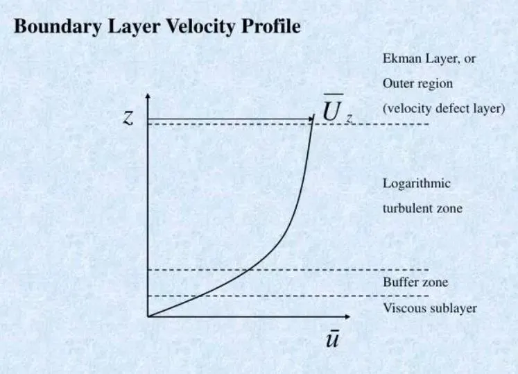
The above picture shows the velocity profile of fluid flowing over a solid body.
As shown, the first layer which is just above the surface is called viscous sub layer.In this layer, viscous effects are dominant. The frictional effects between the fluid layers are high and are responsible for drag and lift forces.
Most of the heat transfer and frictional drag takes place in this layer.
This layer has the highest gradients of velocity, pressure and temperature. Shape of velocity profile in this region is governed by viscosity of fluid.
The top layer is called the log law layer where turbulence effects are high. Turbulent effects dominate the viscous effects. Here, inertial forces are more.
The layer between these two layers is called the Buffer layer where both viscous and turbulent effects are important.
So, to get the correct drag and lift forces, the viscous sub layer must be resolved properly.
There are two approaches to solve the near wall modelling problems. Before that,
1. Viscous sub layer approach: In this approach, the area surrounding the near wall region must be resolved using a very fine mesh.
The parameter that is to be considered to determine whether the mesh is fine or not is call "y+".
It is a dimensionless number and is given by formula
y+ = ((distance from surface to nearest to element) * (wall shear stress)) / (kinematic viscosity)
Wall shear stress depends on the y+ value. Wall shear stress is generated due to drag force. To get correct value of drag force, y+ value should be correct.
As the gradients are high in the near wall region, mesh needs to be fine to get the correct values of flow parameters.
To obtain correct values,
a. y+ value should be approximately 1.
b. Inflation layer growth rate should be 1.2 or less.
c. There should be sufficient number of inflation layer from wall to boundary layer.
Then this mesh is suitable to resolve gradients present in this region.
2. Wall functions approach - In this approach, large no. of cells that needs to be created to resolve the near wall region is replaced with a single cell that has a non-linear function (called as wall function).
The first grid point is located in the log law region of boundary layer and certain wall functions are used to impose suitable conditions close to wall without having to resolve viscous sub layer using fine mesh.
This way, cell count can be reduced and computational time and power can be saved.
y+ value in this approach should be
30 < y+ < 300
But this approach has few limitations. This approach is valid for attached flows and for relatively simple geometry like flat plates or channel flows. Also, this approach is not valid when the Reynolds number is too low but flow is still turbulent.
It is better to use first approach especially in problems involving flow separation and heat transfer.
In this problem, wall functions approach is used for solving.
Preprocessor and Solver setting:
Geometry creation:
Given geometry is below
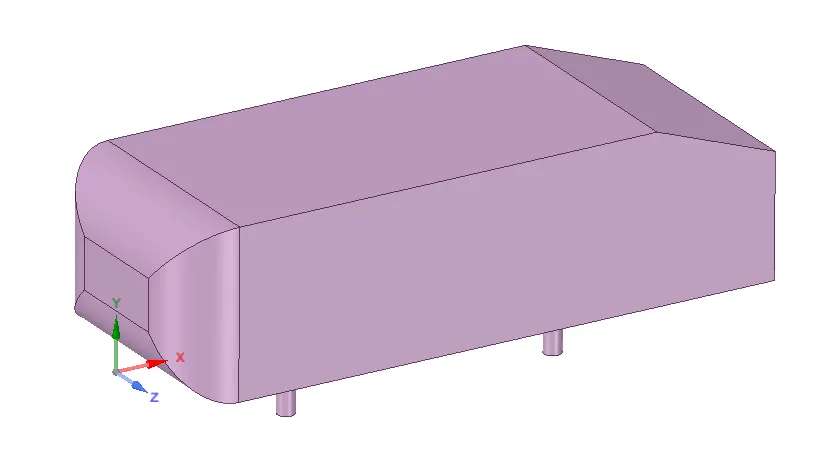
Since the body is symmetrical to X axis, it can be simulated using half of the body and the results would be same for the other half. By doing this, no. of cells can be reduced which reduces computational power and time
This can be done using the "split body" command in spaceclaim.

Select it and select the body which we want to split.
After that, select plane of split and click on the region to disappear.
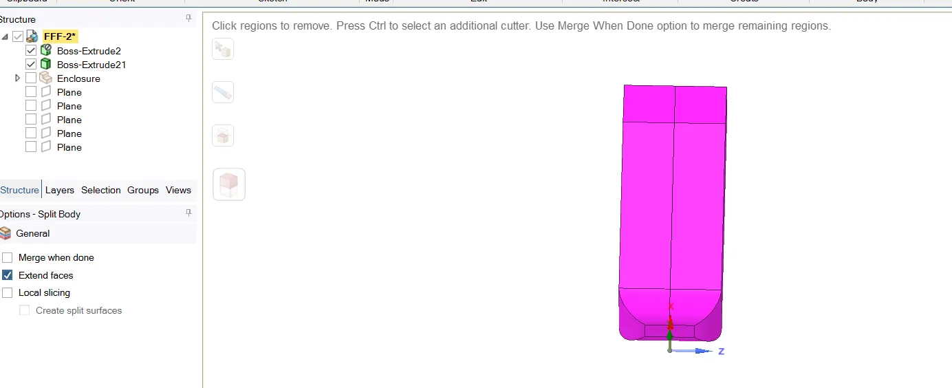
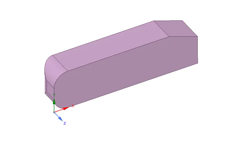
In this problem, as the flow is external i.e., flow takes place over the ahmed body, computational domain needs to be created and meshing is to be done on that domain. Meshing should not be done on the ahmed body as we are not interested in the internal stresses/flow.
A computational domain can be created using option called "Enclosure".
This creates an enclosure over the ahmed body and its dimensions are shown below
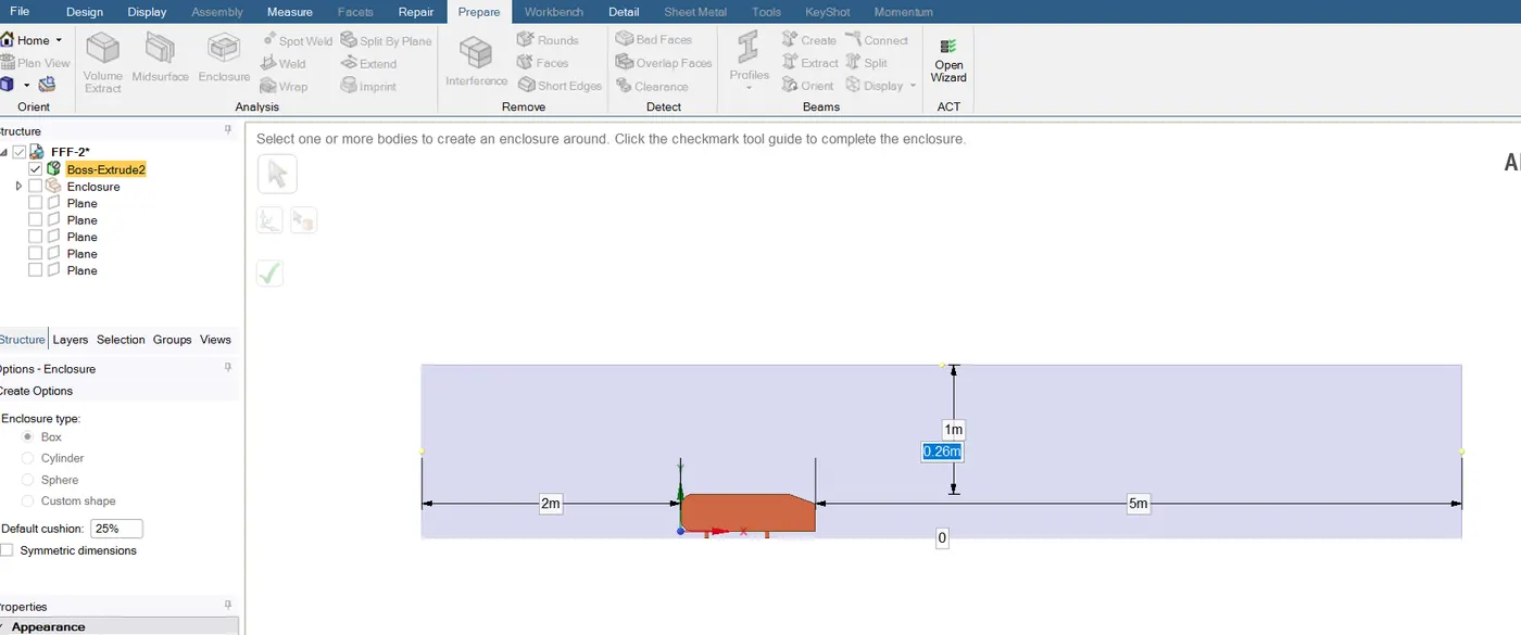
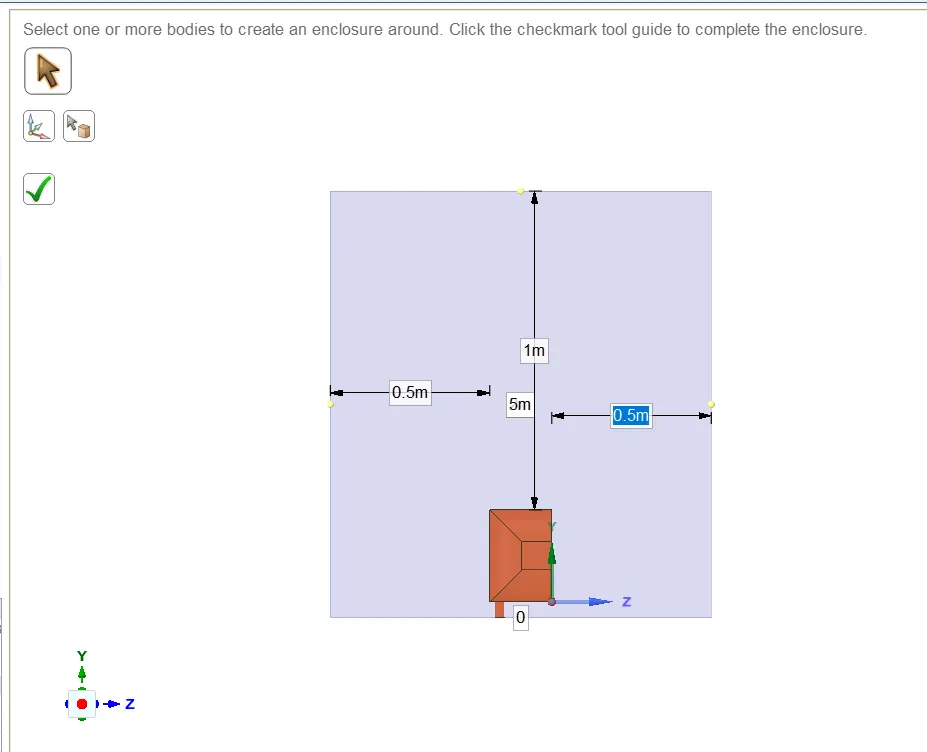
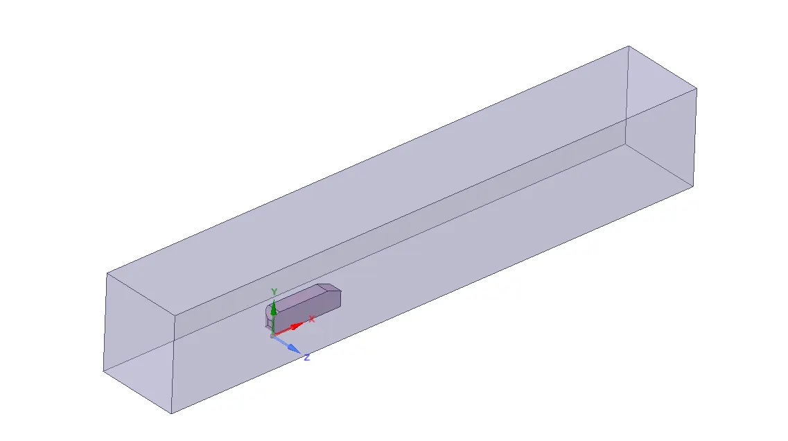
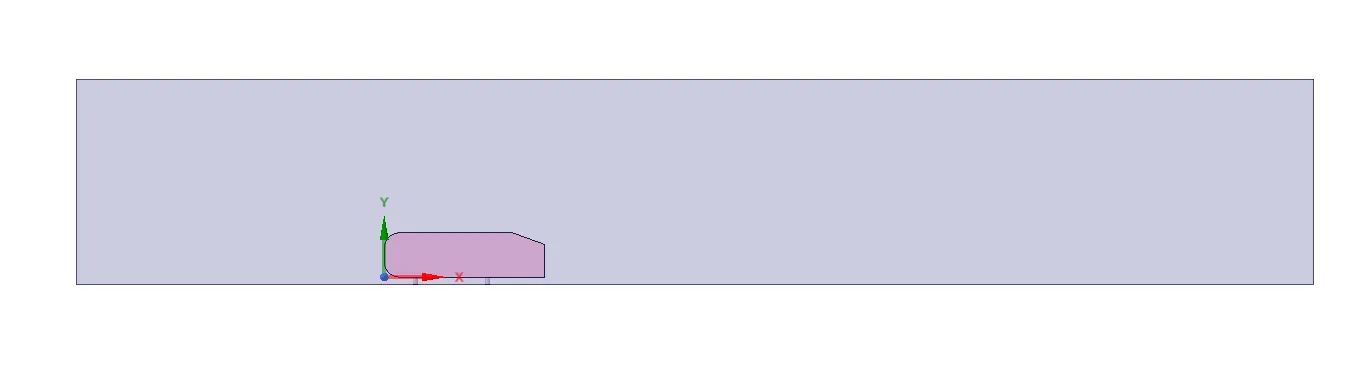
The enclosure is created around the ahmed body and now there are two bodies. But for simulation, just the profile of ahmed body is required but not its solid structure.
Suppress the ahmed body and by default, spaceclaim while creating the enclosure, deleted the intersecting region. In this case, the intersecting region is ahmed body.
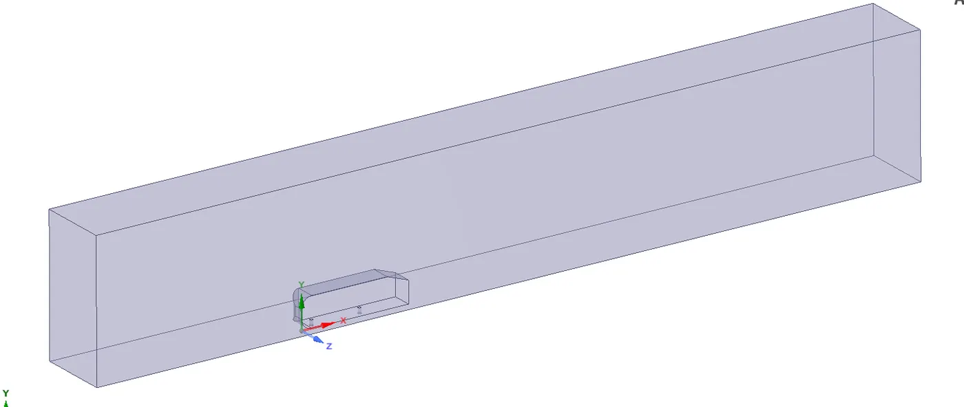
A section view is taken to show the deleted region of ahmed body as below
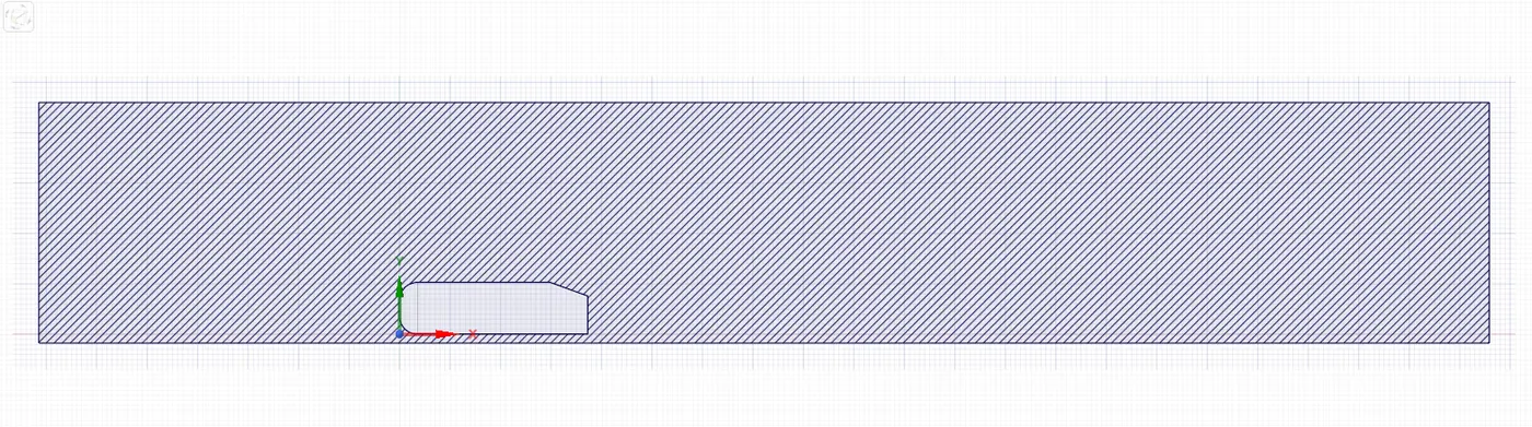
Now mesh can be done on the above domain.
As discussed in solving approach, flow parameter gradients are large near the wall region. So, in order to get those results accurately, mesh resolution around the wall should be fine. Local mesh refinement should be done around the ahmed body region.
To do that, another enclosure smaller in size should be created around the ahmed body. Its dimensions are given below.
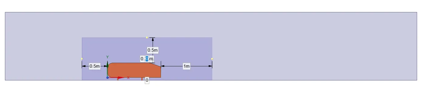
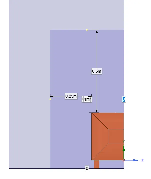
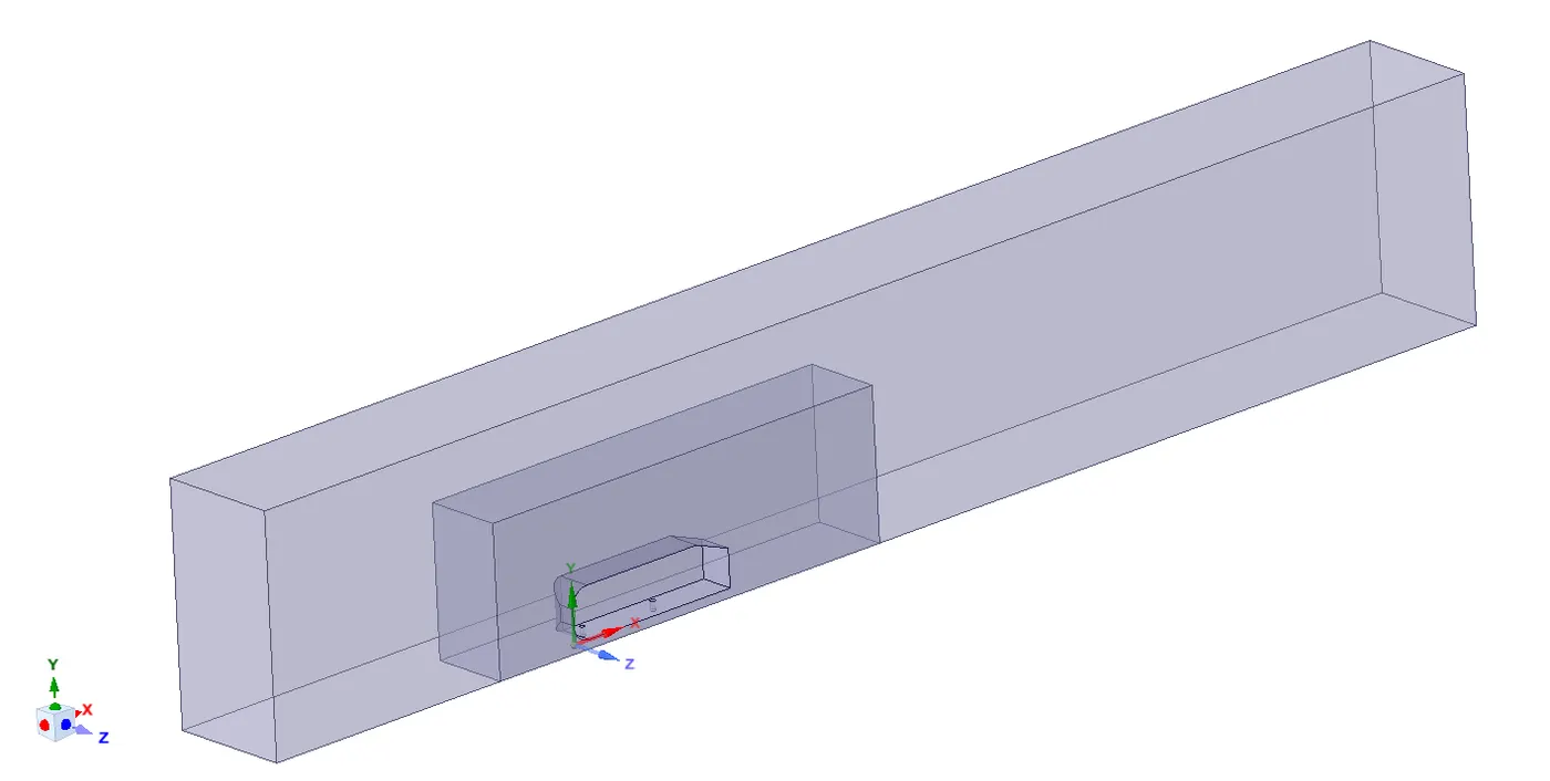
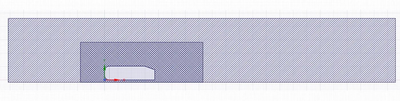
As seen from above section view, the hatches from big enclosure is intersecting with hatches from smaller one which indicates that there is an interference.
To confirm this, do interference check.
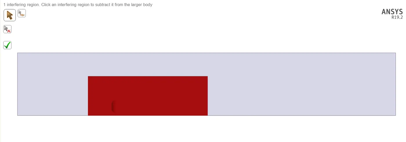
The highlighted area is common in both the enclosures. There should be no interference otherwise the mesh would be improper.
Delete the interference area by clicking in "tick" symbol.
After doing that, check in section view again.
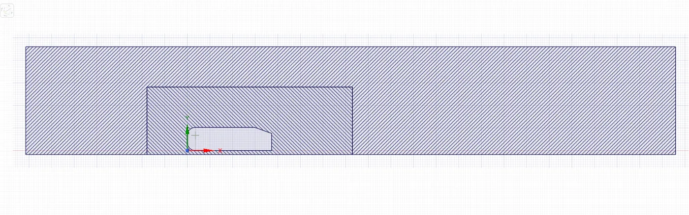
Now, it can be seen that hatches are not intersecting indicating no interference.
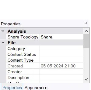
Also, enable "Share topology" in enclosure properties for both the enclosures. This enables the information share between both of them.
Meshing:
Before creating mesh, assign names to regions for which boundary conditions need to be applied.
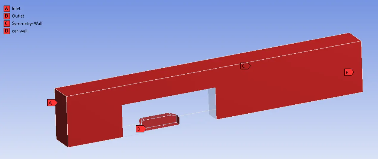
Initially, use the tetrahedral mesh with a size of 0.1 m on the whole model.
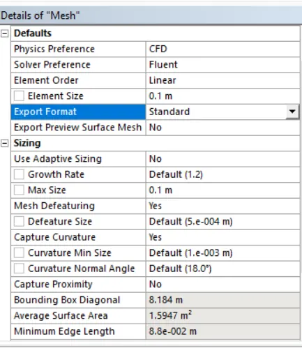
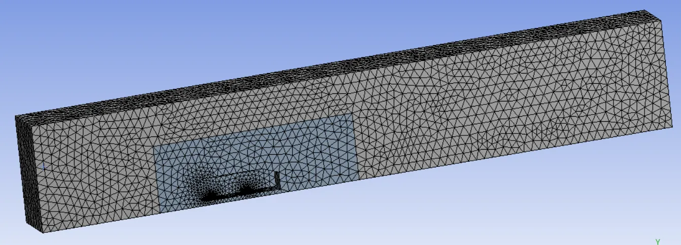
As the outer enclosure does not have any complex geometry, it is better to use hexahedral mesh on that. Hexahedral mesh is of high quality and it must be used whenever possible. But it is better to not use it for complex shapes like the inner enclosure.
Select mesh and insert option "Method" and choose option "Multizone".
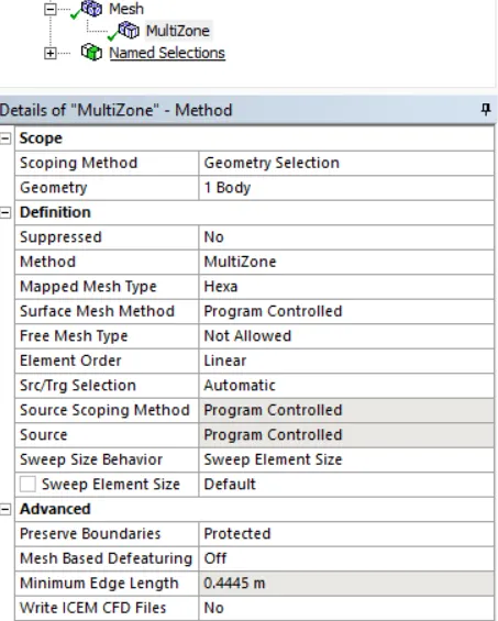
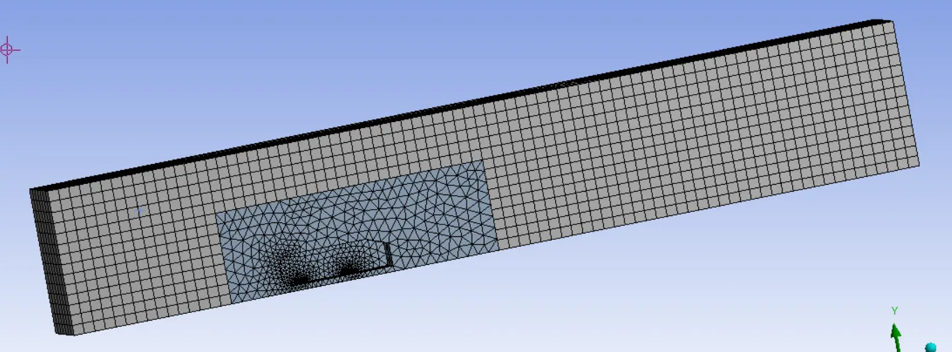
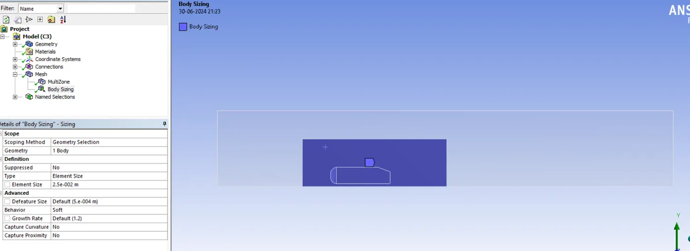
Now the mesh of inner enclosure is to be refined. As we have created if for the purpose of capturing large gradients of flow parameters, it is good to have fine mesh in it.
For this, use option "Sizing" in mesh and select the inner enclosure. The mesh element size is taken as 0.025m.
Inner enclosure after the mesh refinement
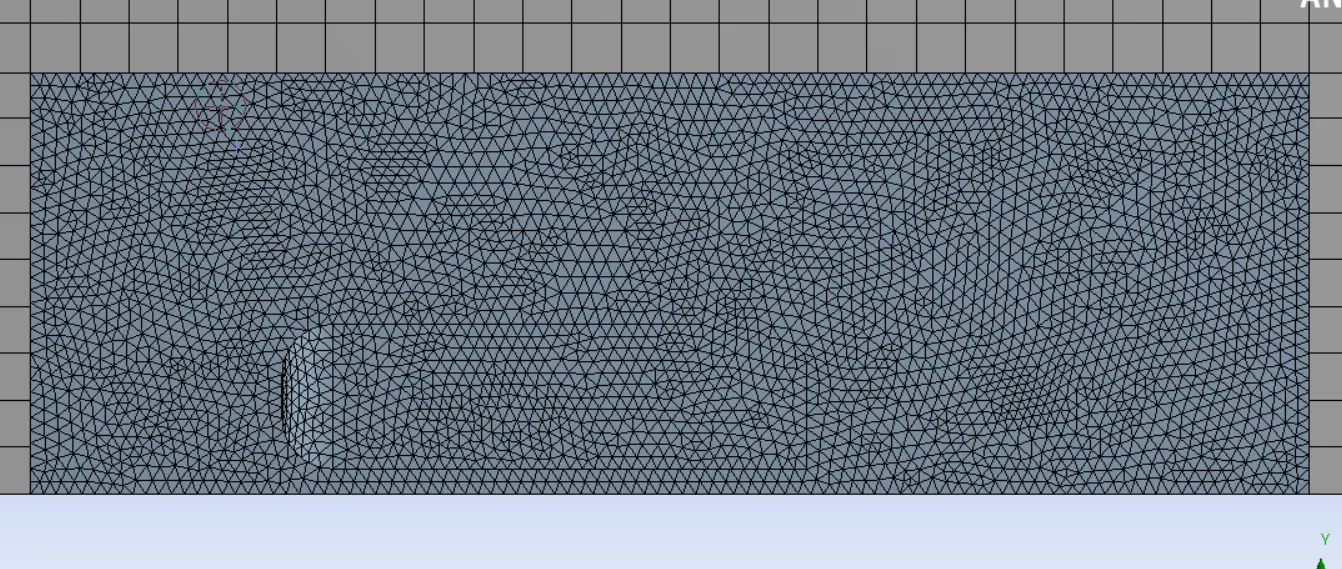
After creating this mesh, it is observed that two protrusions at the bottom are not proper. They do not resemble their original circular shape.
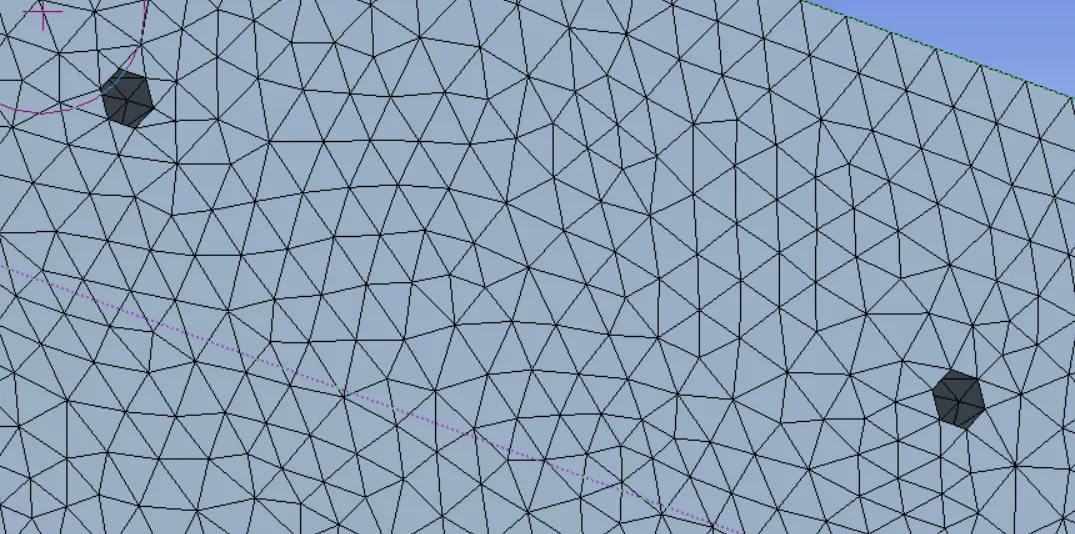
This is an error and should be resolved. For this, again sizing option is selected and face sizing is done for these two protrusions. The mesh element size is further refined to 0.0025m to obtain circular shape.
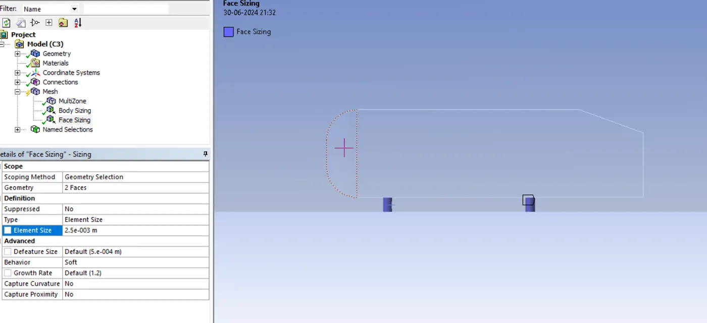
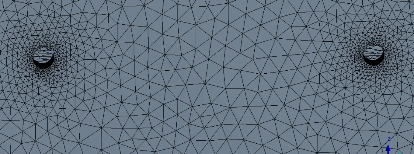
As seen from above picture, circular shape is achieved for the two holes and the mesh size is adjusted for nearby elements.
As said from previous solver section, wall functions approach is used for solving. In this approach, y+ value should be anywhere between 30 and 300.
In this problem, y+ value is taken as 30.
The first grid point should be located in the log law region of boundary layer.
For this, the distance from the wall to the first cell must be obtained for a y+ value of 30.
It can be calculated from various online calculators.
One such is shown below taken from website
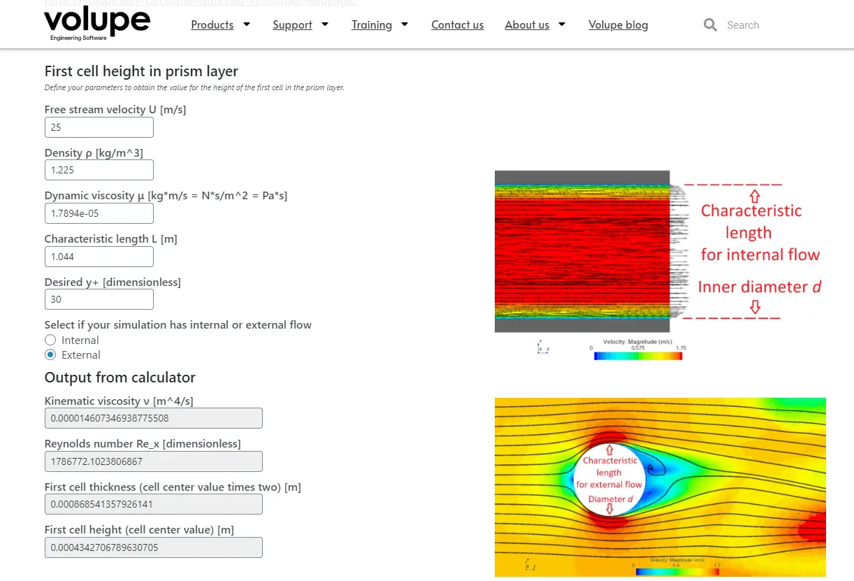
One such is shown below taken from website by giving free stream velocity, density, dynamic viscosity and y+ values as input, the first cell height (distance between wall and first grid point) is obtained.
In this case, the distance is 0.0004342 m.
For creating an element which should be at the above distance, "inflation layers" are used.
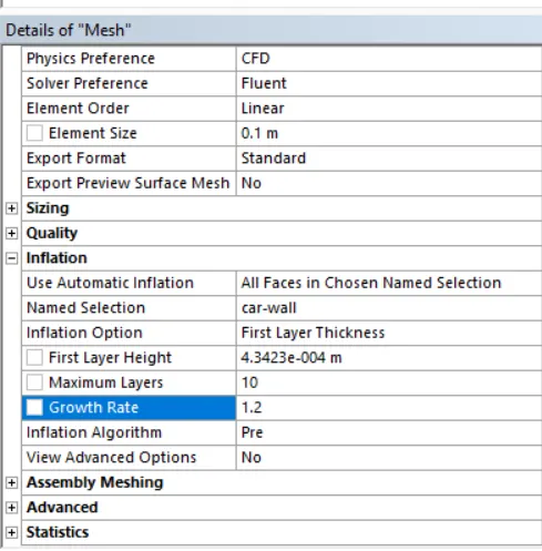
The layers should be around the car wall.
Inflation option is selected as "first layer thickness".
The first layer height is given as 0.0004342m.
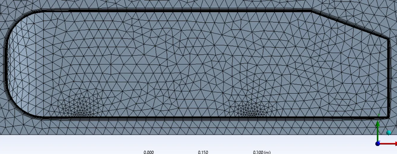
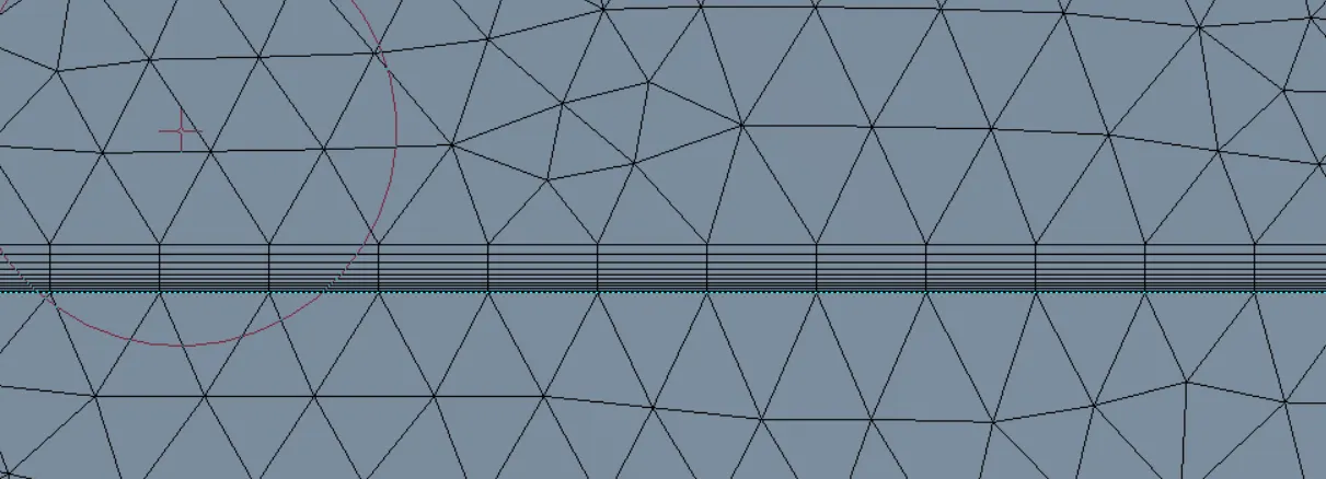
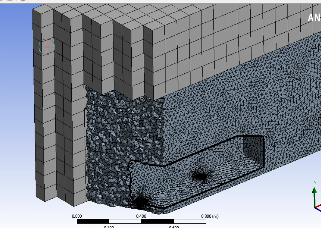
Final meshed model:
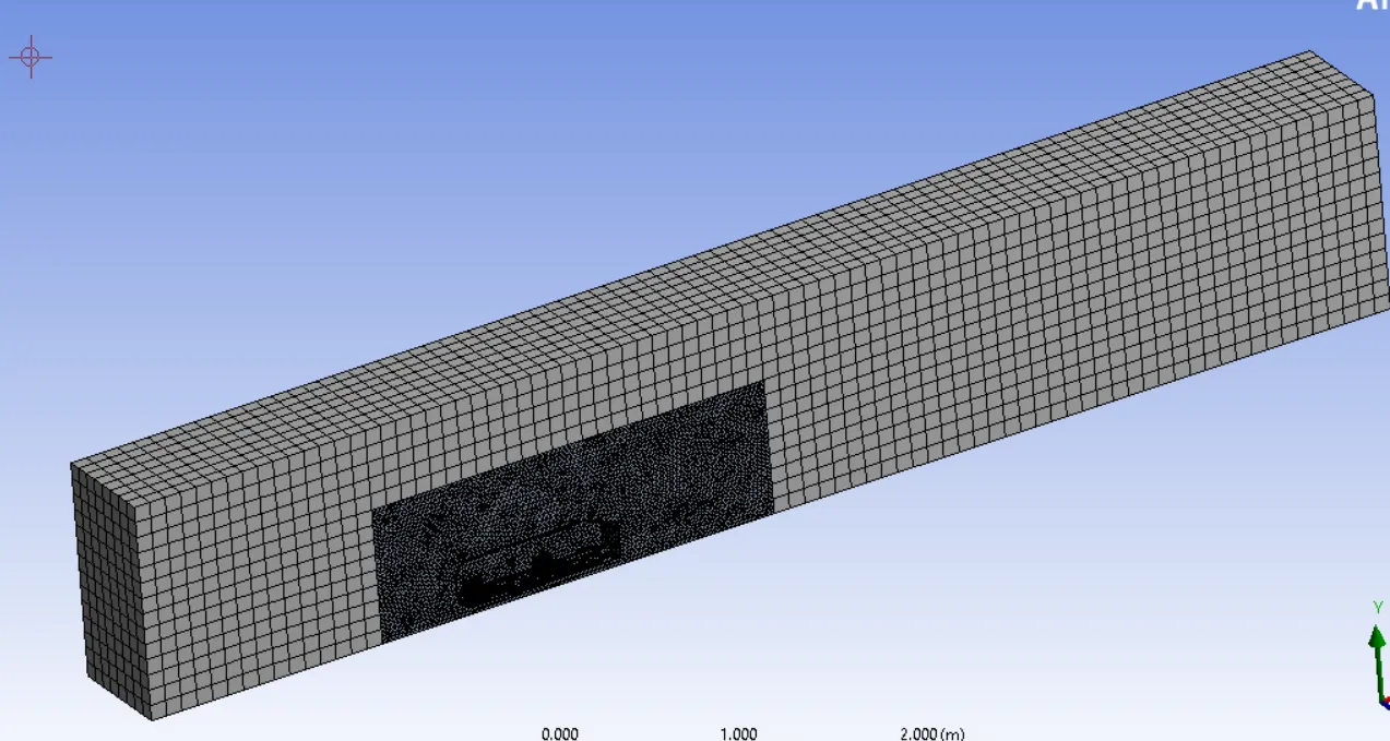
Section view of the meshed body
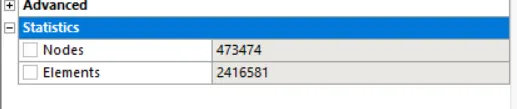
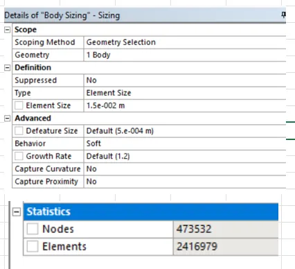
No. of nodes and elements are given below
Solver setting:

Steady state solver is selected.
For the given velocity of 25 m/s, as the match number is less than 0.3, pressure based solver is selected.
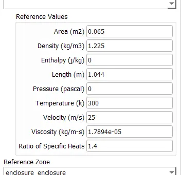
Reference values are as below
Air is selected as the fluid.
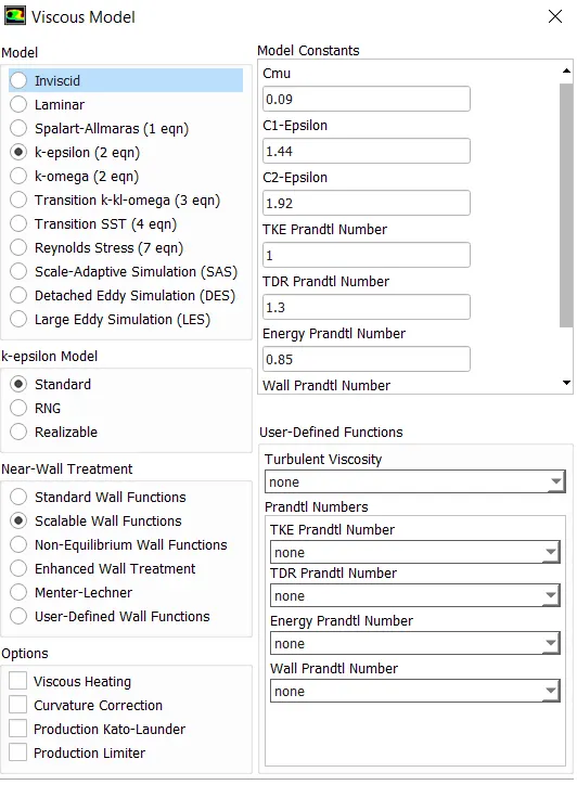
The turbulence model used is k-epsilon with scalable wall functions.
Next boundary conditions are assigned.
For the inlet, velocity of 25 m/s and temperature of 300k.
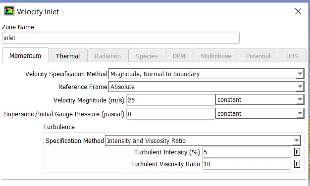
The outlet is assigned a pressure boundary condition with gauge pressure of 0 and temperature of 300K.
The car wall is assigned as a stationary wall with no slip condition.
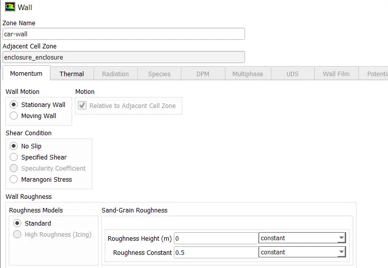
The symmetry wall is assigned with symmetry boundary condition.

Hybrid initialization is performed and solution is run for 300 iterations.
Drag, lift, velocity, pressure and residual profiles are plotted.
Results & Conclusions:
1. Drag plot -
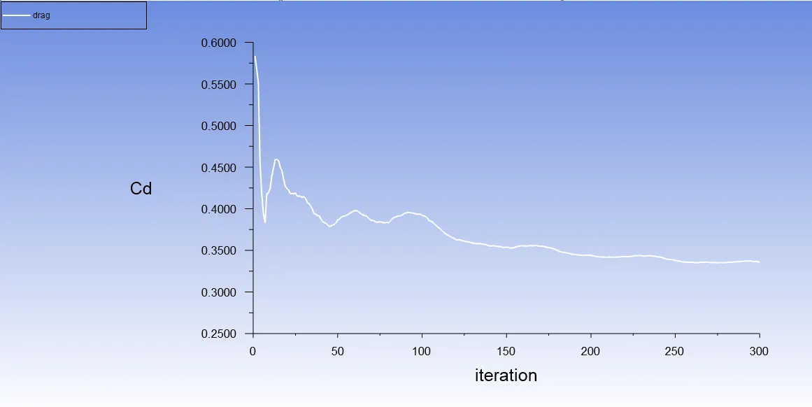
Drag on the car wall is around 0.33
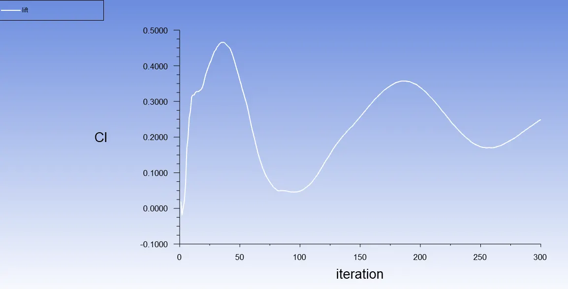
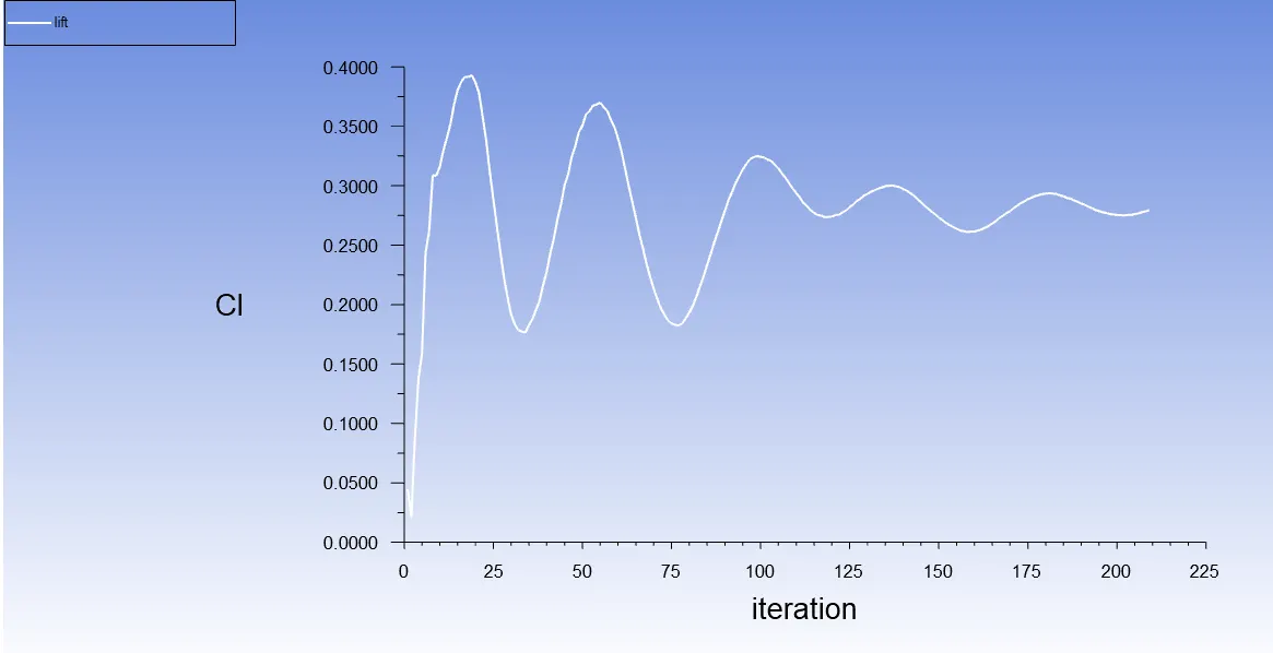
2. Lift plot -
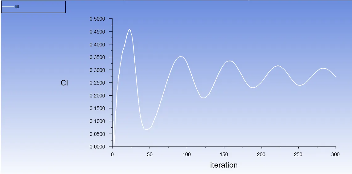
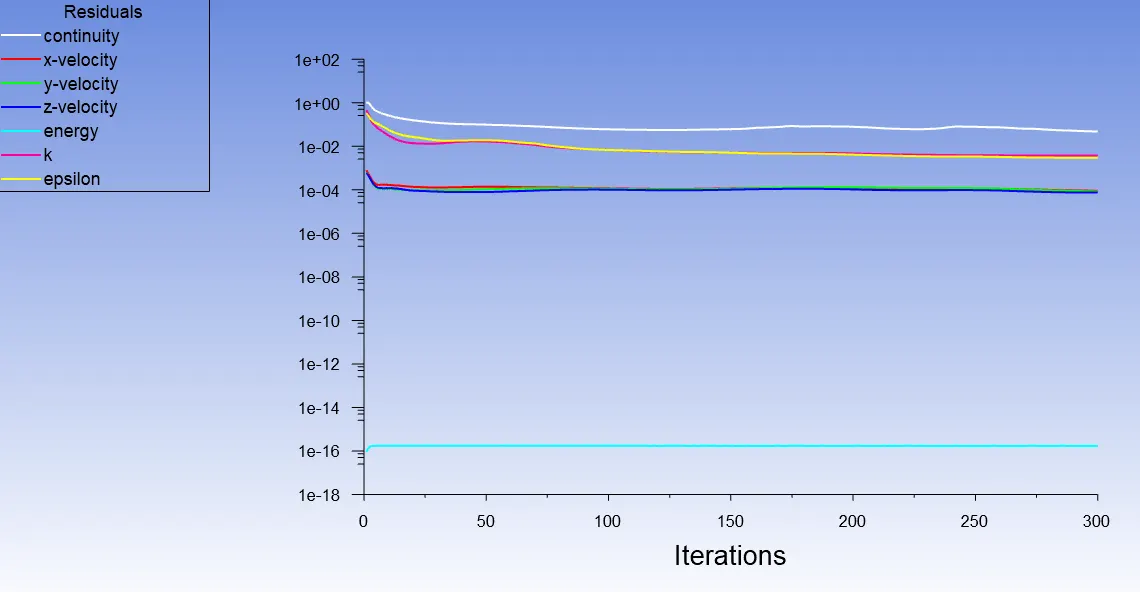
3. Residuals -
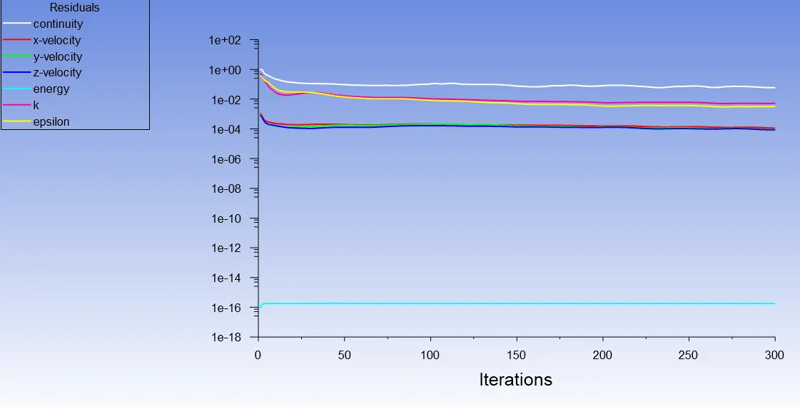
As seen from above plot, convergence is achieved.
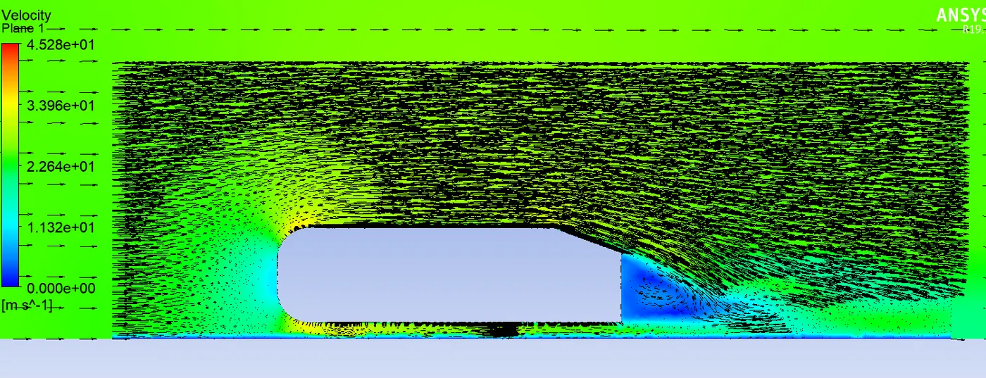
4. Velocity contour at a section plane -
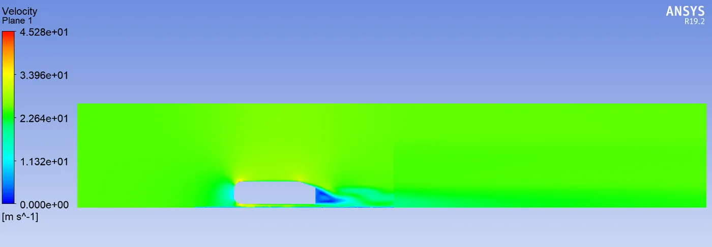
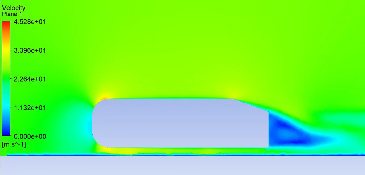
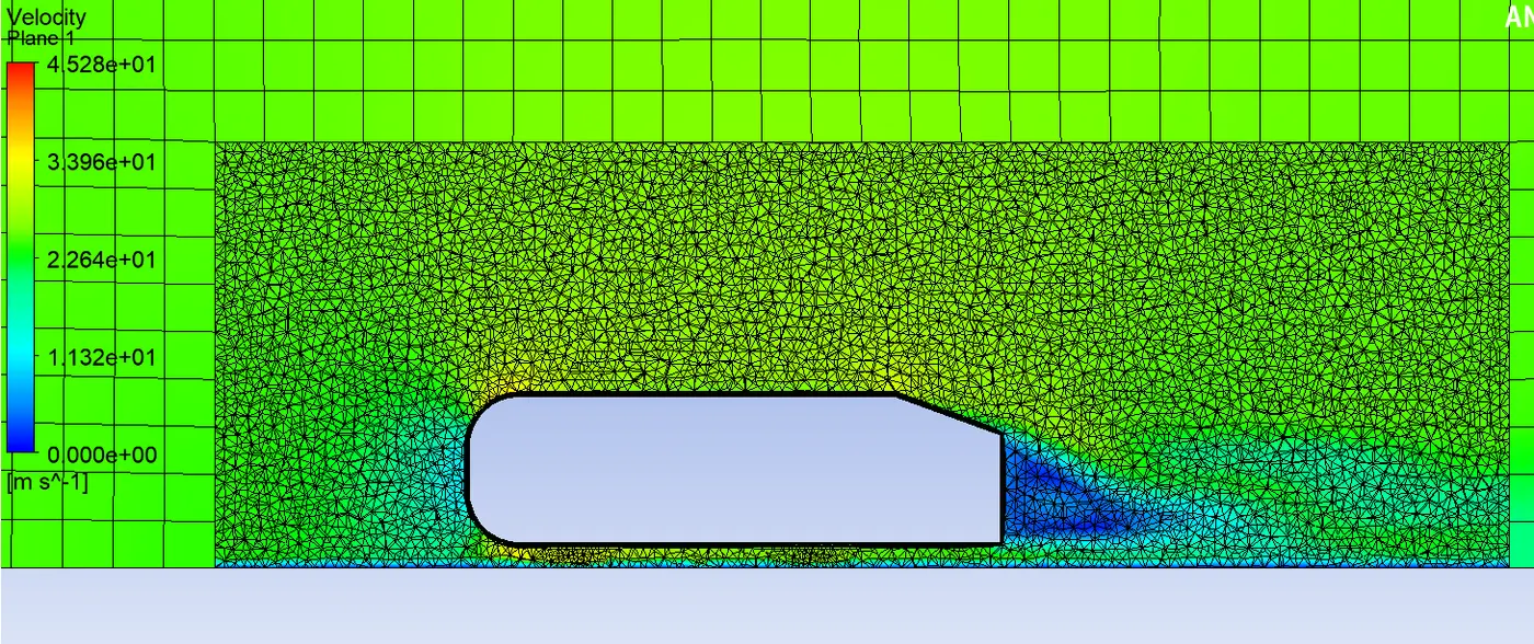
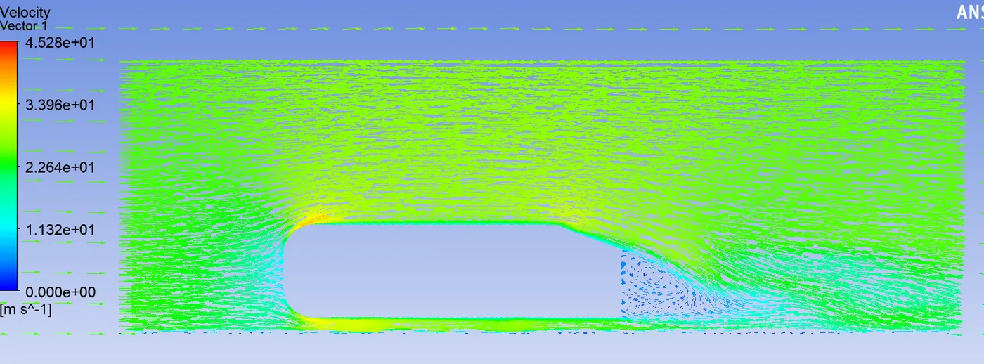
With velocity vectors
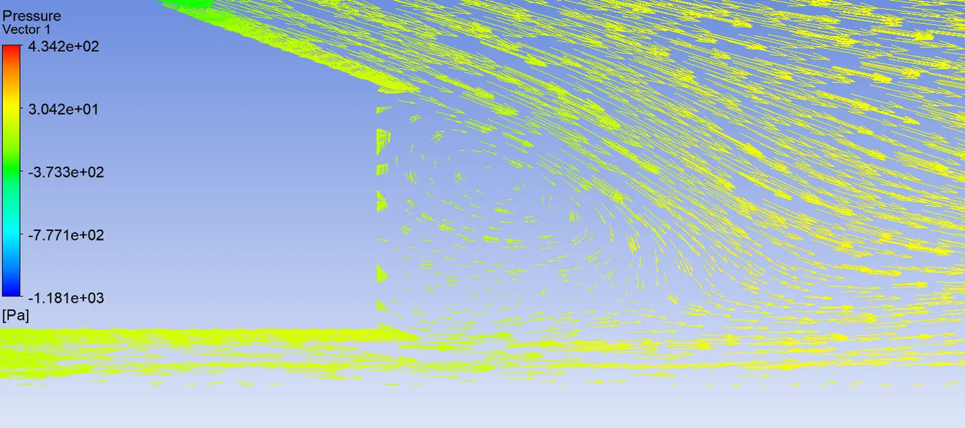
Flow at wake region
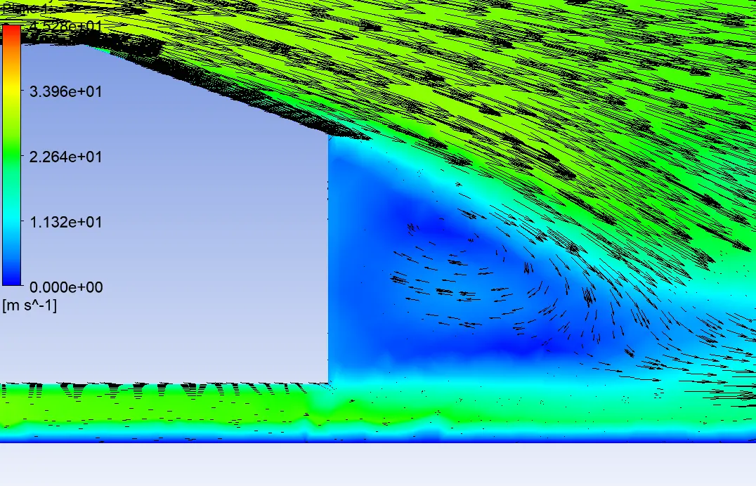
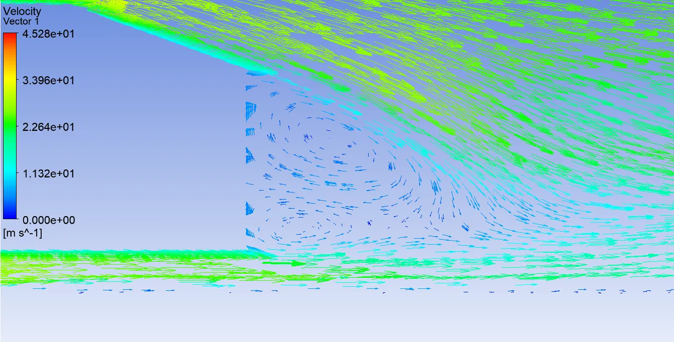
From above pictures, it is observed that the velocity is minimum in the wake region (just behind the ahmed body). Velocity is maximum at the front of the body.
The fluid velocity near the surface of ahmed body is around 22 m/s and gradually reached to free stream velocity of 25 m/s going up. The region where the flow velocity is minimum near the surface till it reaches free stream velocity is called Boundary layer region.
It can be seen that the flow is recirculating behind the body. A region of turbulence is formed where the fluid is trying to move into the wake region.
This happens because the flow is getting separated.
5. Pressure contour -
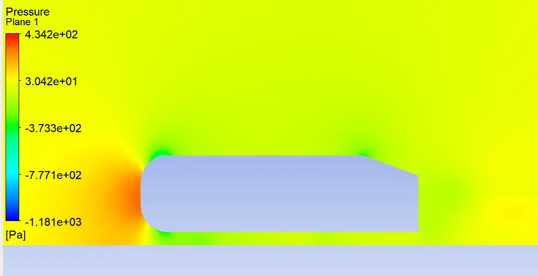
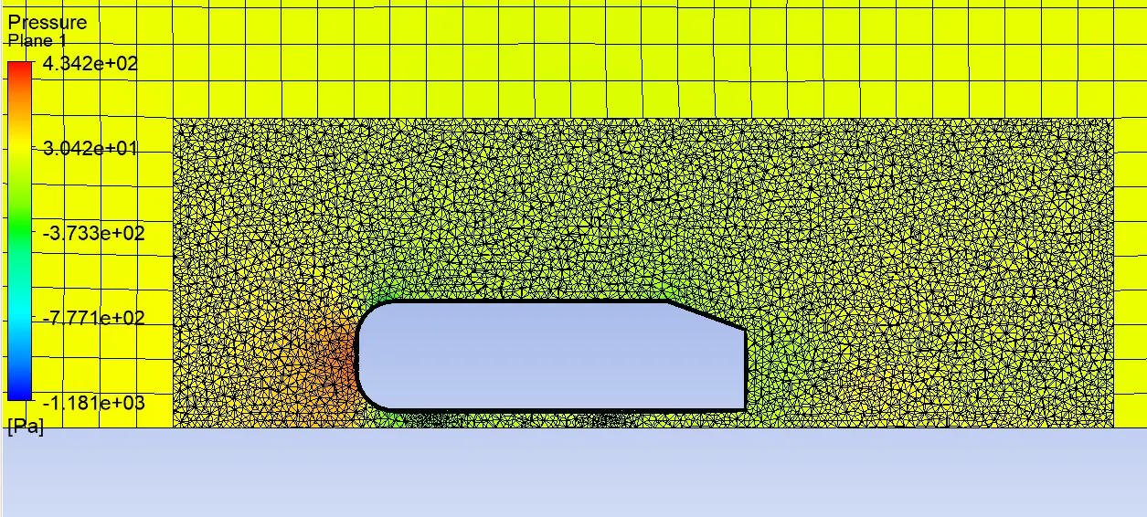
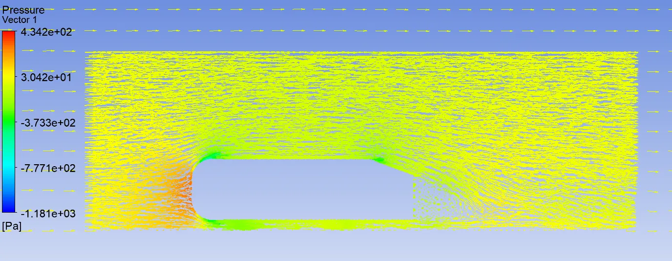
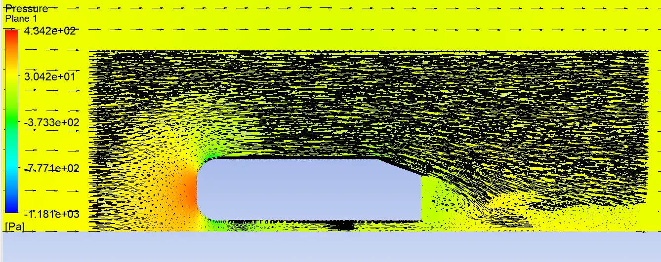
From the above plots, it can be seen that the pressure is high at the front of the body and low(negative) just behind the body (wake region).
Since the curvature is flat and vertical at the front, fluid molecules hit the surface and thereby pressure increases which increase the drag. So, more force is required to overcome this drag and thereby more fuel is consumed.
This can be avoided if the front curvature is stream lined i.e., curvature should be in such a way that it matches the flow of fluid.
Negative pressure is observed at the back of ahmed body. Due to this, fluid molecules are trying to move into this region and flow recirculation is happening.
This negative pressure is created because the flow is getting separated. The flow behind an object separates from the surface and it creates a turbulent region called wake. Pressure in this region remains low due to the flow separation.
As the fluid is moving over the body, it sticks to the body forming a boundary layer. This is called attached flow. There exists a point where the flow begins to separate from the body due to its curvature ( at sharp transitions). Here the boundary layer lifts off. this point is called separation point. After this point, flow becomes separated and this leads to increase in pressure drag thereby increasing the overall drag.
The design of any structure moving through a fluid should be such that the flow remains attached to it for a long time and the separation point must be as low as possible. This creates less turbulence and avoids the formation of wake region thereby reducing drag and vortices.
Grid Independence Study:
The mesh independence study is done on this setup ( on the inner enclosure) to find if the same results can be obtained with different element sizes.
Normal study is done with element size of 0.025m.
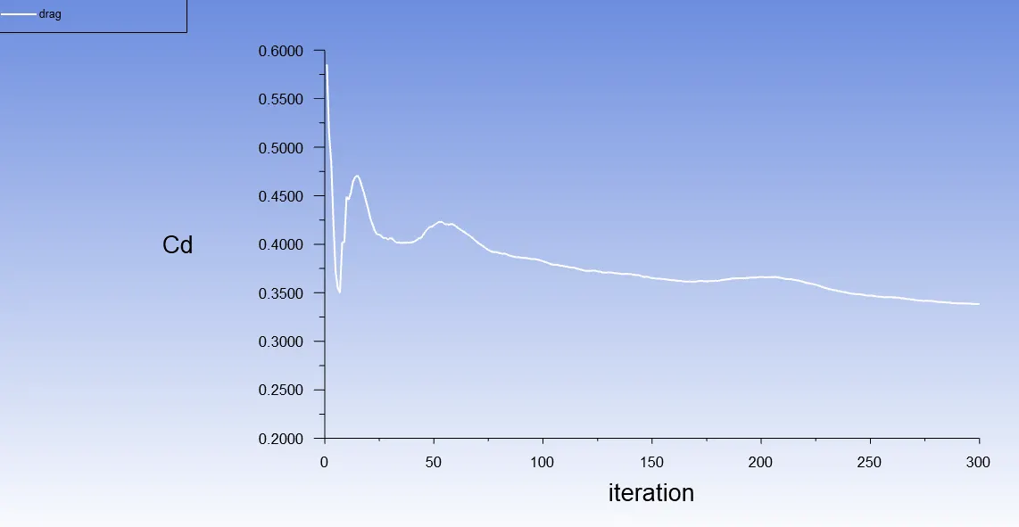
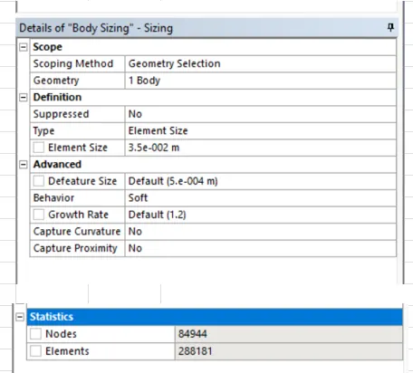
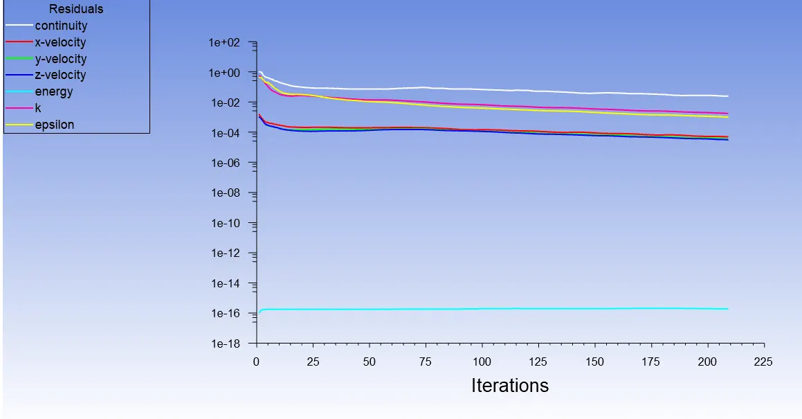
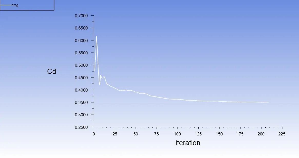
Mesh independence study is done with two element sizes - 0.015 and 0.035m.
| element size 1- 0.015m | Normal study - 0.025m | Element size 2- 0.035m | |
| no. of nodes | 473532 | 473474 | 84944 |
| no. of elements | 2416979 | 2416581 | 288181 |
Results of element size 1 -0.015m
Results of element size 2 -0.035m
Summary:
| Element size 1- 0.015m | Normal study - 0.025m | Element size 2- 0.035m | |
|---|---|---|---|
| Drag | 0.33 | 0.33 | 0.35 |
| Lift | 0.25 | 0.275 | 0.275 |
From the above study, it is observed that the lift and drag values for both the element sizes of 0.015m and 0.035m closely match with normal study results.
So, it can be concluded that the setup has mesh independence in normal study.