Week 3 - External flow simulation over an Ahmed body.

Objective:-

The Aerodynamic behaviour of a Ahmed body is numerically investigated in the present work by using the Commerical Software ANSYS FLUENT for the simulation using a Turbulent model. In this case we are considering the only half Ahmed body for the best practice where you can save on the number of cells and get the results faster as well.

Also, the Grid dependency test is performed to validate the results against the experimental data and compute the coefficient of drag and lift maintaining the y+ in the appropriate range.

Problem Statement:-

1. Describe Ahmed's body and its importance.

2. Explain the reason for the negative pressure in the wake region. 

3. Explain the significance of the point of separation. 

Expected Results:

1. Velocity and pressure contours.

2. The drag coefficient plot for a refined case.

3. The vector plot clearly showing the wake region. 

Theory:-

The Ahmed body is a generic car body (a simplified vehicle model). The airflow around the Ahmed body captures the essential flow features around an automobile and was first defined and characterized in the experimental work of Ahmed. Although it has a very simple shape, Ahmed body allows us to capture characteristic features that are relevant to bodies in the automobile industry.

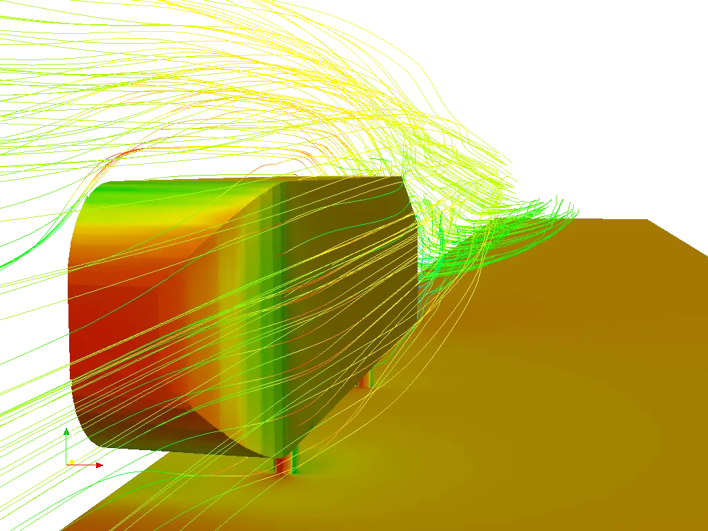
This model is also used to describe the turbulent flow field around a car-like geometry. Once the numerical model in validated, it is used to design new models of the car. So, it becomes a benchmark for aerodynamic simulation tools. The aim of the benchmark validation was to evaluate the ANSYS, computational fluid dynamics (CFD) software, and compare its results with the measurement data. The particular goal of this benchmark is to compare the Drag Coefficient, Velocity Profiles, Velocity field, and the time-averaged Wake structure of the ANSYS simulation results with the real experimental measurement in the wind tunnel.

Modelling Approach:-

The Flow for this case we are using is Turbulent flow which is based on the Reynolds number means the Re >2000 for this flow and turbulent model is k-epsilon. The K-epsilon model is used for the High reynolds number, Steady, Equilibrium flows without a large adverse pressure gradient explicity modelling the effect of the innermost portion of the turbluent layer is not neccesary.In this challenge we are using Ahmed body.The Ahmed body represents a simplified, ground vehicle geometry of a bluff body type. Its shape is simple enough to allow for accurate flow simulation but retains some important practical features relevant to automobile bodies. This model describes how to calculate the turbulent flow field around a simple car-like geometry using the Turbulent Flow, k-epsilon interface.

Here, is the given geometry of the Ahmed body that we are consider for validating the simulation.

2D Geometry of Ahmed Body:-

The simple geometrical shape has a length of 1.044m, height of 0.288m and width of 0.389m. The shape of cylinderical pillars that is attached to the bottom of the body has a dimension of 0.5 m and the slant height of the rear surface ϕ=30°.The Ahmed body with the slant angle of 25° belongs to the fastback vehicles, which exhibit very strong inward rotating longitudinal vortices at the C-pillars.

These vortices extend far into wake and generate a field of downwind in the enclosed region. At slant angle of 30 degrees, i.e, directly before transition to the full squareback flow, this pair of vortices is devolped most strongly, and the flow separates at the lower edge of the stant. This produces strong under-pressures at that position, So that the aerodyanmic drag reaches its maximum in this state here, is the 3D model of the Ahmed body.

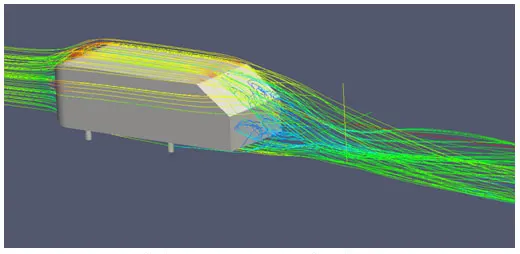
The flow for this model we are consider is Turbluent which is based on the Reynold's number determined by the body length and the inlet velocity. The simulation solves for the turbulent kinetic energy and dissipation on addition to the velocity and pressure fields.

Solution Approach:-

Step1 Creating a Geometry

In this case we are going to load a geomtery in ANSYS FLUENT space claim from a stp file format.

The Ahmed body is enclosed by a virtural wind tunnel created by an enclosure option in prepare toolbox. In this case first we split the body in half part for fastest convergence as mentioned in the above. Then create a virtual fluid domain by an enclosure option and uncheck the symmtery for the editing the required dimensions. 

We have created a 2 enclosure boxes the inner one is for add local refinement region right in front of Ahmed body and also in the wake region.

The outer one is for fluid domain where we need to know the flow features around a body So, we need to create a mesh on the body not inside the body.

Step2:- Meshing

After opening the Mesh set up First we creates name by selection command like inlet, outlet, symmetry and car walls .

After that we create first the baseline mesh of element size is 100mm and generate the mesh For the hexahedral we have to go insert sizing and select the multizone for the different different mesh patterns. It will generate hexahedral baseline automatically.  

For the local refinement region mesh size we are using it 50mm for beacuse the as the mesh is more finer the more accurate the result It will captures the flow behaviour at every point. Right click on the mesh go to insert option and then select the sizing option. Select the inner box then give the element size 50mm and generate mesh.

Here, we introduce the Important term Y+ 

• It is important to know about the concept of wall  Y+ or in general how the flow behaves near the wall, to consider the effects near the wall as it is the basis on which choice of the turbulence model is governed.
• The behaviour of the flow near the wall is a complicated phenomenon and to distinguish the different regions near the wall the concept of wall Y+ has been formulated. Thus  is a dimensionless quantity, and is distance from the wall measured in terms of viscous lengths.
• One of the reasons for the need of Y+ is to distinguish different regions near the wall or in the viscous region, however how exactly it helps in turbulence modelling or in general CFD modelling need to be well understood.
• The concept of Y+ , and based on the  Y+ value the first cell height can be calculated. The near wall region is meshed using the calculated first cell height value with gradual growth in the mesh so that the effects are captured and avoiding overall heavy mesh count.
• It provides a relation between frictional velocity Ut , absolute distance from the wall to cell (y) and kinematic viscosity(rho/mhu)
• The y+ value is a non-dimensional distance (based on local cell fluid velocity) from the wall to the first mesh node, as you can see in the image below.  To use a wall function approach for a particular turbulence model with confidence, we need to ensure that our y+ values are within a certain range.

Let us see how to calculate first cell height. Firstly, we should calculate the Reynolds number for our model based on the characteristic scales of our geometry.

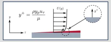
If the Y+ value is less than 5 the solver uses viscous sublayer equation and the y+ value is greater than 30 to 200 the solver uses log-law emprical equation automatically we dont need to set up the relationships between u+ and Y+ given below in the graph.

The curve in red line is the DNS called direct numerical solution shows the relationshipe between u+ and y+ here, is the calculation for the first cell height on the basis of assuming Y+ value bascially y+ value tells where our mesh lies.

  Reynold's number(Re) = (rho*v*L)/ μ`

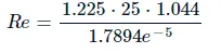
Re = 17.8677e^5

             skin friction (Cf ) = 0.079*Re^-0.2    for external flows                    

             cf = 0.0032                                                            (after putting value of Re number)

             Shear stress at wall (τwall)= 0.5*cf*rho*v^2

              τwall  = 1.2389 N/m^2                                         (after putting value of cf and rho)

            frictional velocity Ut =√(τwall/rho)

Ut = 1.00567m/s^2

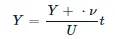
Let us asumme Y+ = 240 we got y = 3.5 mm from this formula similarly, Y+ = 342 we got y = 5mm and Y+ = 410

<!-- [if !supportLists]-->·         <!--[endif]-->Now to add the body fitted mesh on the surface of the Ahmed body for this we use the inflation layer command Then go to inflation. Select geomerty from named selection choose car wall. Type of inflation layer is Total thickness. Give the no. of layers and total thickness based on first layer thickness. click on Generate mesh.

    

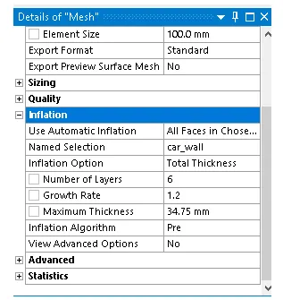
Here, we are Calculate the total thickness on the basis of first cell height we got from the assumed Y+ value bascially Y+ value tells where our mesh lies So, the total thickness of the inflation layer is

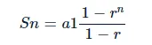
a1 = first term of first layer of thickness

r=growth rate 

n= no. of layers 

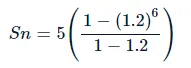
Sn = 34.75mm

Step3 Start Fluent Setup

Select Density-Based solver because It solves for high speed incompressible flows whose Mach no. is greater than 0.3. It solves Energy, momentum, continuty and species transport equations simultaneously. 

      

     Viscous model is selected as K- Epsilon model. Wall treatment standerd.

       

             

       Now, to plots the velocity and pressure contours in the fluid domain or over the Ahmed body first we have to create a plan in the xy direction at the z=0 then create reports of velocity and pressure contours

     

    After the complete data set up first we do the initialzation In this case we are using the hybrid initilazation because It solves for potential flow probelms and also provides good initial conditions. Method we are using in this case is SIMPLE implicit method.

   

 

• After the initilazation the problem go in Run and calculation type the number of iterations as you want to run number of times your simulation and then hit calculate.
• Step4 Results 
•  
• Iteration convergence plot - Residual plot 

     

       Coeffcient of drag 

 

  

       Coeffcient of lift

   

 

    Velocity Contour 

     

 

    Pressure contour

        

     Vectors

 

     

 

    Graph of velocity profile at different locations of y

 

 

     Grid Independce test:

     In this study we have set about 4 cases, by refining the mesh and varriation in the Y+ values to check the effect on Coefficient of drag and lift values.

 

Y+ value	1st cell thickness (in mm)	Total thickness (in mm)	Baseline Mesh size (in mm)	No of layers	Coefficient of Drag	Coefficient of Lift
240	3.5	34.75	50	6	0.34715	0.2533
240	3.5	34.75	25	6	0.3030	0.2409
342	5	49.64	50	6	0.34914	0.23258
410	6	59.75	50	6	0.34922	0.2864

 

    Case1:   y+ = 240  mesh size = 50mm

 

     Iteration convergence plot - Residual 

     

Coeffcient of Lift 

Velocity contour 

 

Pressure contour 

Vectors 

Vectors in 3D show wake region

Graph of velocity profile at different locations of y

Case2:  y+ = 342  and mesh size = 50mm

Iteration convergence plot - Residual 

Coeffcient of drag 

Coeffcient of Lift

Velocity contour 

Pressure  contour 

Vectors 

Vectors show wake region

 Graph of velocity profile at different locations of y

Case4 : y+ = 410  and mesh size = 50mm 

Iteration convergence plot - Residual 

Coefficient of Drag 

Coefficient of Lift

Velocity contour 

Pressure contour 

Vectors

Vectors in 3D show wake region

 Graph of velocity profile at different locations of y

Case4 : Y+ = 240  and mesh size = 25mm

Iteration convergence plot - Residual 

Coeffcient of drag

Coeffcient of Lift

Velocity contour

Pressure contour

Vectors

Vectors 3D show wake region

 Graph of velocity profile at different locations of y

 

      Conclusion:-

      We can clearly conclude that In the wake region the velocity is high as compared the velocity in the backside i.e, tail region and the Velocity vectors is also very high in the wake region It is because the obstruction offered by an Ahmed body in the wake region is more as compared in the tail region. In the Tail region of the Ahmed body the circulating flow is more that results in low velocity.The pressure in the front is very high but in the wake region we got is Adverse pressure or called negative Pressure and here, we got the term Negative pressure 

     Negative Pressure Gradient:

     When an object moves in a fluid the fluid sticks on the surface of the body and formed a boundary layer over it. Now, for certain bodies and type of motion , there is a point on the body where the fluid detaches from its surface, thus breaking the boundary layer, this point at which fluid detaches from the surface is called flow of separation. The boundary layer maintains till the velocity gradient is greater than zero and when the velocity gradient goes decrease or negative The flow of separation takes place.

     Flow seperation

     

   

•       In this case flow seperation takes place at the curved surface interface of the Ahmed body. Separation occurs due to an adverse pressure gradient and also negative velocity gradient encountered as the flow expands and its resulting in the recirculating flow.
•      The coefficient of drag and the lift is increases when the of y+ value is increases and also when the mesh is finer the coefficient of drag and lift is also less that is because the larger initial y+ value, smaller overall mesh count and faster run times. Expect flow separation and the accurate prediction of the separation point will have an impact result, such as the drag or lift forces experienced by the ellipse then would be advised to resolve the boundary layer all the way to the wall with a finer mesh.
•      The residuals continously dropping as we refining the mesh with the Y+ value means the error is significantly reduced.
•      The flow separation and apprearence of vortices gets more prominent as Y+ is increased by refining the mesh wake region is captured properly.
•     From the pressure contours we can clearly see that the pressure at the frontal area is more and also the velocity is less at the frontal area.