Week 3.5 - Deriving 4th order approximation of a 2nd order derivative using Taylor Table method

AIM:

To derive the fourth order approximations of a second order derivative using central differencing scheme, skewed right sided difference and skewed left sided difference with the help of taylor table method and to compare the analytical derivative with obtained values for the given function.

GOVERNING EQUATIONS

CENTRAL DIFFERENCING SCHEME:

The number of nodes = p+q-1

Where, p is order of derivative.

q is order of approximations.

The no of nodes = 2+4-1 =5.

DERIVATION

To derive a fourth order approximation for the second order derivatrive,we can start with these approximation,

`(∂ ^2 u)/ (∂ x^ 2) = (a f ( i − 2 ) + b f ( i − 1 ) + c f ( i ) + d f ( i + 1 ) + e f ( i + 2 ) )/(d x^ 2)` .....................(1)

taylor series derivation for above terms,

`a f ( i − 2 ) = a f ( i ) − (2 a f ' ( i ) d x)/ (1 !) + (4 a f ' ' ( i ) d x ^ 2)/(2 !) + (8 a f ' ' ' ( i ) d x^3)/( 3 !) + (16 a f ' ' ' ' ( i ) d x^4)/ (4 !)` ............................(2)

Similarly expand all the terms in the equation(1) and are represented in the form of table using taylor table method

`d x^2 f ' ' ( i )`	`f(i)`	`f ' ( i ) d x`	`f ' ' ( i ) d x ^2`	`f ' '' ( i ) d x ^3`	`f ' ''' ( i ) d x ^4`
`af(i-2)`	a	-2a	2a	`(-4a)/3`	`(-2a)/3`
`bf(i-1)`	b	-b	`b/2`	`-b/6`	`(b)/24`
`cf(i)`	c	0	0	0	0
`df(i+1)`	d	d	`d/2`	`d/6`	`d/24`
`ef(i+2)`	e	2e	2e	`(4e)/3`	`(2e)/3`
sum of co_efficients	0	0	1	0	0

the linear equation obtained from the above table are solved using matrix inversion method,

A.X=B

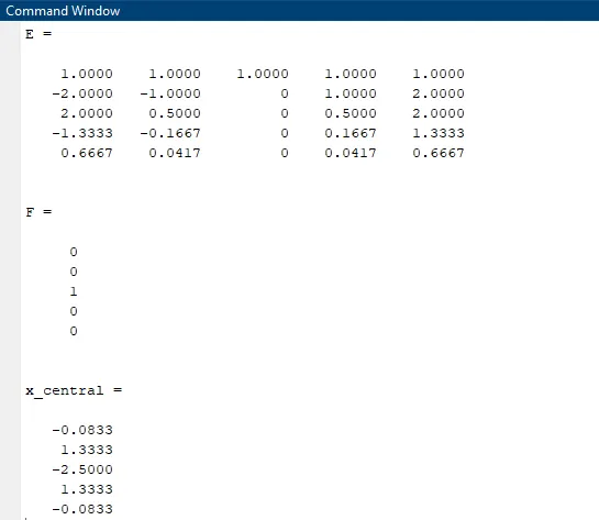
sustituting these coefficient in equation(1) we get,

`(∂^ 2 u)/ (∂ x^ 2) = (( − 0.0833 ) f ( i − 2 ) + ( 1.3333 ) f ( i − 1 ) + ( − 2.5000 ) f ( i ) + ( 1.3333 ) f ( i + 1 ) + ( − 0.0833 ) f ( i + 2 ))/ (d x ^2)`

SKEWED RIGHT HAND DIFFERENCE SCHEME:

The number of nodes = p+q

Where, p is order of derivative.

q is order of approximations.

The no of nodes = 2+4 =6.

DERIVATION:

To derive a fourth order approximation for the second order derivative,we start with these approximation,

`(∂^2 u)/ (∂ x^ 2) = (a f ( i ) + b f ( i + 1 ) + c f ( i + 2 ) + d f ( i + 3 ) + e f ( i + 4 ) + g f ( i + 5 ) )/(d x^2)`

Similarly expand all the terms in the equation and are represented in the form of table using taylor table method'

`d x^2 f ' ' ( i )`	`f(i)`	`f ' ( i ) d x`	`f ' ' ( i ) d x ^2`	`f ' '' ( i ) d x ^3`	`f ' ''' ( i ) d x ^4`	`f ' ''' ( i ) d x ^4`
`af(i)`	a	-5A	`(25a)/2`	`(-125a)/6`	`(625a)/24`	`(3125)/120`
`bf(i+1)`	b	-4b	`(16b)/2`	`(64b)/6`	`(256b)/24`	`(1024b)/120`
`cf(i+2)`	c	-3c	'(9c)/2`	`(27c)/6`	`(81c)/24`	`(243c)/120`
`df(i+3)`	d	-2d	`(4d)/2`	`(8d)/6`	`(16d)/24`	`(32d)/120`
`ef(i+4)`	e	-e	`(e)/2`	`(-e)/6`	`(e)/24`	`(e)/120`
`gf(i+5)`	g	0	0	`0`	0	0
sum of co_efficients	0	0	1	0	0	0

the linear equation obtained from the above table are solved using matrix inversion method,

A.X = B

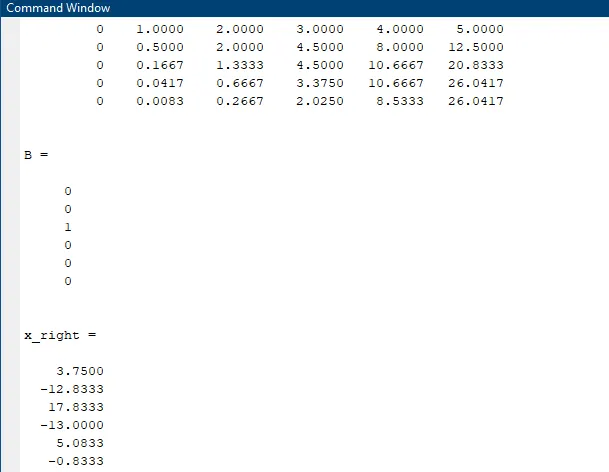
substituting these coefficient in equation(2) we get,

`(∂^2u)/(∂x^2)=((3.7500)f(i)+(−12.8333)f(i+1)+(17.8333)f(i+2)+(−13.0000)f(i+3)+(5.0833)f(i+4)+(−0.8333)f(i+5))/(dx^2)`

SKEWED LEFT HAND DIFFERENCE SCHEME:

The number of nodes = p+q

Where, p is order of derivative.

q is order of approximations.

The no of nodes = 2+4 =>6.

DERIVATION:

To derive a fourth order approximation for the second order derivative,we start with these approximation,

`(∂ ^2 u)/( ∂ x^ 2) = (a f ( i − 5 ) + b f ( i − 4 ) + c f ( i − 3 ) + d f ( i − 2 ) + e f ( i − 1 ) + g f ( i ) )/(d x^2)`

expand all the terms in the equation using taylor series expansion and are represented in the form of table using taylor table method.

`d x^2 f ' ' ( i )`	`f(i)`	`f ' ( i ) d x`	`f ' ' ( i ) d x ^2`	`f ' '' ( i ) d x ^3`	`f ' ''' ( i ) d x ^4`	`f ' ''' ( i ) d x ^4`
`af(i)`	a	0	0	0	0	`0`
`bf(i+1)`	b	b	`b/2`	`b/6`	`(b)/24`	`(b)/120`
`cf(i+2)`	c	2c	'(4c)/2`	`(8c)/6`	`(16c)/24`	`(32c)/120`
`df(i+3)`	d	3d	`(9d)/2`	`(27d)/6`	`(81d)/24`	`(243d)/120`
`ef(i+4)`	e	4e	`(16e)/2`	`(64e)/6`	`(256e)/24`	`(1024e)/120`
`gf(i+5)`	g	5g	`(25g)/2`	`(125g)/6`	`(625g)/24`	`(3125g)/120`
sum of co_efficients	0	0	1	0	0	0

the linear equation obtained from the above table are solved using matrix inversion method,

A.X = B

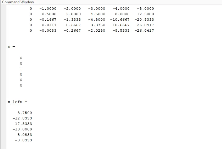
`(∂^ 2u)/ (∂ x^ 2) =( ( − 0.8333 ) f ( i − 5 ) + ( 5.0833 ) f ( i − 4 ) + ( − 13.0000 ) f ( i − 3 ) + ( 17.8333 ) f ( i − 2 ) + ( − 12.8333 ) f ( i − 1 ) + ( 3.7500 ) f ( i ) )/(d x^2)`

MATLAB PROGRAM

Function for central difference 4th order error at particular spacing 'dx'

%Function program for Central differnce 4th order error at particular
%spacing x

%% Create function for the 4th order approximation using cetrnal differnce

function error_central_differncing=central_differnce(x,dx)
%Analytical funcction f(x)=exp(x)*cos(x)
%f''(x)=-2*exp(x)*sin(x)

analytical_derivative=-2*exp(x)*sin(x);

%% values of coefficients calculated from taylor table

E = [1, 1, 1, 1, 1;-2, -1, 0, 1, 2;4/2, 1/2, 0, 1/2, 4/2;-8/6, -1/6, 0, 1/6, 8/6;16/24, 1/24, 0, 1/24, 16/24];
F = [0;0;1;0;0];
x_central =inv(E)*F;

a=x_central(1)
b=x_central(2)
c=x_central(3)
d=x_central(4)
e=x_central(5)

%% numerical derivative using taylopr table central differncing scheme
%central differencing;
%(d^2u/dx^2)/dx^2=
%((a*f(x-2*dx)+(b*f(x-dx))+(c*f(x))+(d*f(x+dx))+(e*f(x+2*dx))/dx^2;
%central differnece fourth order approximation

central_differencing_fourth_order_approx=((a*exp(x-2*dx)*cos(x-2*dx))+ ...
(b*exp(x-dx)*cos(x-dx))+(c*exp(x)*cos(x))+(d*exp(x+dx)*cos(x+dx))+ ... 
    (e*exp(x+2*dx)*cos(x+2*dx)))/dx^2;

error_central_differncing=abs(central_differencing_fourth_order_approx-analytical_derivative);
end

Function for skewed right sided difference 4th order error at particular spacing 'dx'

%SKEWED RIGHT SIDED DIFFERNCE
%Function program for skewed right sided differnce 4th order error at particular spacing x

%% Create function for the 4th order approximation using cetrnal differnce

function error_skewed_right_sided=skewed_right_sided(x,dx)

%Analytical funcction f(x)=exp(x)*cos(x)
%f''(x)=-2*exp(x)*sin(x)

analytical_derivative=-2*exp(x)*sin(x);

%% values of coefficients calculated from taylor table

A = [1 1 1 1 1 1;0 1 2 3 4 5;0 1/2 4/2 9/2 16/2 25/2;0 1/6 8/6 27/6 64/6 125/6;0 1/24 16/24 81/24 256/24 625/24;0 1/120 32/120 243/120 1024/120 3125/120];
B = [0;0;1;0;0;0];
x_right = inv(A)*B;

a=x_right(1)
b=x_right(2)
c=x_right(3)
d=x_right(4)
e=x_right(5)
g=x_right(6)

%% numerical derivative using taylopr table central differncing scheme
%skewewd right sided differencing;
%(d^2u/dx^2)/dx^2=
%((a*f(x)+(b*f(x+dx))+(c*f(x+2*dx))+(d*f(x+3*dx))+(e*f(x+4*dx)+(g*f(x+5*dx))/dx^2;
%skewed right sided fourth order approximation

skewed_right_sided_fourth_order_approx=((a*exp(x)*cos(x))+(b*exp(x+dx)*cos(x+dx))+ ...
    (c*exp(x+2*dx)*cos(x+2*dx))+(d*exp(x+3*dx)*cos(x+3*dx))+(e*exp(x+4*dx)*cos(x+4*dx))+ ...
     (g*exp(x+5*dx)*cos(x+5*dx)))/dx^2;

error_skewed_right_sided=abs(skewed_right_sided_fourth_order_approx-analytical_derivative);
end

Function for skewed left sided difference 4th order error at particular spacing 'dx'

%SKEWED LEFT SIDED DIFFERNCE
%Function program for left sided differnce 4th order error at particular spacing x

%% Create function for the 4th order approximation using cetrnal differnce

function error_skewed_left_sided=skewed_left_sided(x,dx)

%Analytical funcction f(x)=exp(x)*cos(x)
%f''(x)=-2*exp(x)*sin(x)

analytical_derivative=-2*exp(x)*sin(x);

%% values of coefficients calculated from taylor table

C = [1 1 1 1 1 1;0 -1 -2 -3 -4 -5;0 1/2 4/2 9/2 16/2 25/2;0 -1/6 -8/6 -27/6 -64/6 -125/6;0 1/24 16/24 81/24 256/24 625/24;0 -1/120 -32/120 -243/120 -1024/120 -3125/120];
D = [0;0;1;0;0;0];
x_left = inv(C)*D;

a=x_left(6)
b=x_left(5)
c=x_left(4)
d=x_left(3)
e=x_left(2)
g=x_left(1)
%% numerical derivative using taylopr table central differncing scheme
%skewewd left sided differencing;
%(d^2u/dx^2)/dx^2=
%((a*f(x-5*dx)+(b*f(x-4*dx))+(c*f(x-3*dx))+(d*f(x-2*dx))+(e*f(x-dx)+(g*f(x)))/dx^2;
%skewed left sided fourth order approximation

skewed_left_sided_fourth_order_approx=((a*exp(x-5*dx)*cos(x-5*dx))+(b*exp(x-4*dx)*cos(x-4*dx))+ ...
    (c*exp(x-3*dx)*cos(x-3*dx))+(d*exp(x-2*dx)*cos(x-2*dx))+(e*exp(x-dx)*cos(x-dx))+(g*exp(x)*cos(x)))/dx^2;

error_skewed_left_sided=abs(skewed_left_sided_fourth_order_approx-analytical_derivative);
end

Main program for calculating 4th order error of second-order derivative using central,skewed,right-sided, and skewed left-sided scheme using previously developed functions:

%calculating 4th order error of second-order derivative using central, 
%skewed right sided and left sided scheme;
clear all
close all
clc

x=pi/3;
dx=linspace(pi/4,pi/40000,40);

%creating 'for' loop;
for i=1:length(dx)
    central_difference_error(i)=central_differnce(x,dx(i));
    skewed_right_side_error(i)=skewed_right_sided(x,dx(i));
    skewed_left_side_error(i)=skewed_left_sided(x,dx(i));
end

%plotting graphs for dx vs errors for central,skeweed right sided, & skewed
%left sided approximatioins

figure(1)
plot(dx,central_difference_error,'linewidth',2)
hold on
grid on
plot(dx,skewed_right_side_error,'r','linewidth',2)
hold on
plot(dx,skewed_left_side_error,'g','linewidth',2)
xlabel('dx')
ylabel('error')
legend('Central differnece error','Skewed right-sided error','Skewed  left-sided error')
title('Truncation error vs range of dx')

figure(2)
loglog(dx,central_difference_error,'linewidth',2)
hold on
grid on
loglog(dx,skewed_right_side_error,'r','linewidth',2)
hold on
loglog(dx,skewed_left_side_error,'g','linewidth',2)
xlabel('range of dx')
ylabel('truncation error')
legend('Cenrtal differnce error','Skewed right sided error','skewed left sided error')
title('Truncation error vs range of dx-log graph')

RESULTS

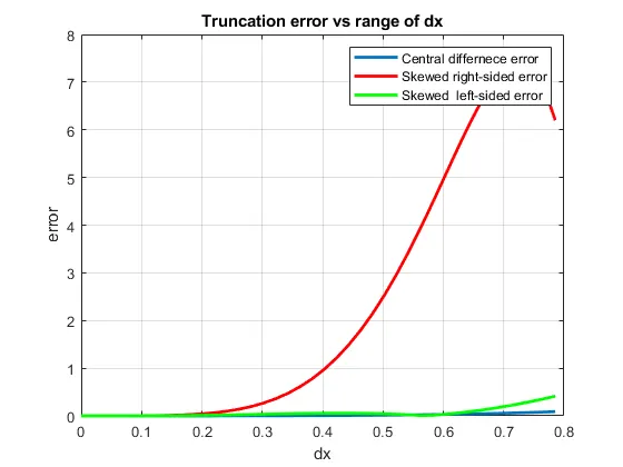
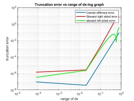
As seen from the plot, the central differencing scheme has very less error compared to other schemes. Therefore, central differencing is better than other schemes because it uses information from both the sides from the point of consideration to give approximative and accurate values.

As the left and right skewed difference methods uses data only from one side of point of interest it gives less approximative and accurate values about the point.

WHY A SKEWED SCHEME IS USEFUL:

The system which doesn’t contain sufficient information on both side of the point of interest. In such cases we cannot use central differencing scheme so skewed scheme is useful in such cases.

WHAT CAN A SKEWED SCHEME DO THAT A CD SCHEME CANNOT DO:

CDS cannot not be employed at the boundary nodes due to unavailability of right and left nodes at the same time. In such cases the skewed differencing scheme is used.