Project 1 - Parsing NASA thermodynamic data

Aim – To parse a data file and plot the required properties by calculation.

Objectives –

1. To extract the 14 coefficients and calculate the specific heat, entropy and enthalpy for all species in the data file.
2. To calculate the molecular weight of each species.
3. To plot Specific heat, Enthalpy and Entropy with local temperature range from low temperature to high temperature for each species.

Introduction –

File parsing refers to how to read the information from particular text file or any type of file and how to store that information in computer program. Sometimes it is very crucial to read the data from external files or data places to include it in calculation. This is done by partially analyzing the data, understand its structure and then representing this data for further calculation by writing a code.

NASA’s thermodynamic data is parsed in this project. Code for parsing is shown below.

Code for Parsing NASA’s thermodynamic data.

clear all
close all
clc

f1=fopen('THERMO.dat','r');    %open file for reading
line1=fgetl(f1);               %Reading header information
disp(line1);
line2=fgetl(f1);               %Reading 2nd line information
disp(line2);
Header=strsplit(line2,' ')     %Split the string stored in the variable line 2 into substrings basesd on delimiter, which in this case is a space('')

R=8.314;                       %Universal gas constant
global_low_temp=str2num(Header{2})
global_mid_temp=str2num(Header{3})
global_high_temp=str2num(Header{4})

%To avoid the next 3 lines
for i=1:3
    info_line=fgetl(f1);
    disp(info_line)
end

%Reading the species block from THERMO data file

for i=1:53
    Line1=fgetl(f1);
    species_desc=strsplit(Line1,' ');
    species_name=species_desc{1};
    
    a=flip(species_desc);
    
    local_low_temp=str2num(a{4});
    local_high_temp=str2num(a{3});
    local_mid_temp=str2num(a{2});
    
    temp=linspace(local_low_temp, local_high_temp,500);
    
    Line2=fgetl(f1);
    a=findstr(Line2,'E');
    Line3=fgetl(f1);
    b=findstr(Line3,'E')
    Line4=fgetl(f1);
    c=findstr(Line4,'E');
    
    % High Temperature coefficients
    a1=str2double(Line2(1:a(1)+3));
    a2=str2double(Line2(a(1)+4:a(2)+3));
    a3=str2double(Line2(a(2)+4:a(3)+3));
    a4=str2double(Line2(a(3)+4:a(4)+3));
    a5=str2double(Line2(a(4)+4:a(5)+3));
    a6=str2double(Line3(1:b(1)+3));
    a7=str2double(Line3(b(1)+4:b(2)+3));
    
    % Low temperature coefficients
    b1=str2double(Line3(b(2)+4:b(3)+3));
    b2=str2double(Line3(b(3)+4:b(4)+3));
    b3=str2double(Line3(b(4)+4:b(5)+3));
    b4=str2double(Line4(1:c(1)+3));
    b5=str2double(Line4(c(1)+4:c(2)+3));
    b6=str2double(Line4(c(2)+4:c(3)+3));
    b7=str2double(Line4(c(3)+4:c(4)+3));
    
    specific_heat= sp_heat_file_pa(a1,a2,a3,a4,a5,b1,b2,b3,b4,b5,temp,local_mid_temp);
    enthalpy=enthalpy_file_pa(a1,a2,a3,a4,a5,a6,b1,b2,b3,b4,b5,b6,R,temp,local_mid_temp);
    entropy=entropy_file_pa(a1,a2,a3,a4,a5,a7,b1,b2,b3,b4,b5,b7,R,temp,local_mid_temp);
    Mw=molecular_weight_file_pa(species_name);
    
    figure(1)
    plot(temp,enthalpy,'linewidth',2,'color','b');
    title('temp vs enthalpy',species_name)
    xlabel('temperature')
    ylabel('Enthalpy')
    grid on
    
    figure(2)
    plot(temp,entropy,'linewidth',2,'color','r')
    title('temp vs entropy',species_name)
    xlabel('temp')
    ylabel('entropy')
    grid on
    
    figure(3)
    plot(temp,specific_heat,'linewidth',2,'color','y')
    title('temp vs specific heat',species_name)
    xlabel('temp')
    ylabel('specific heat')
    grid on
    
    mkdir(species_name);
    %directory=(['D:skill lync',species_name]);
    cd(species_name);
    
    saveas(1,'enthalpy.jpg')
    saveas(2,'entropy.jpg')
    saveas(3,'specific_heat.jpg')
    cd ..
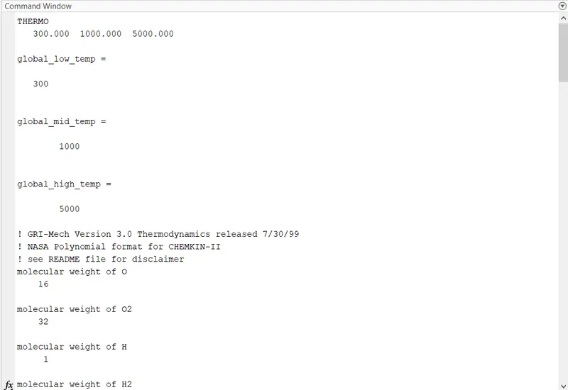
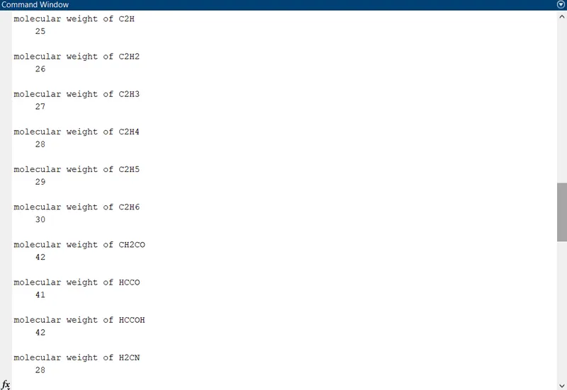
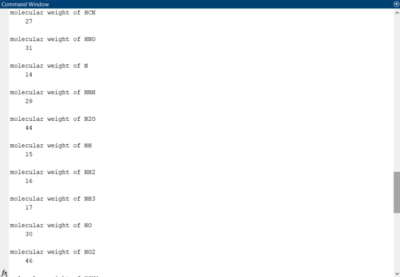
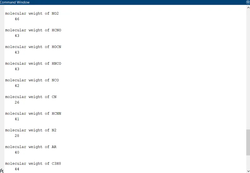
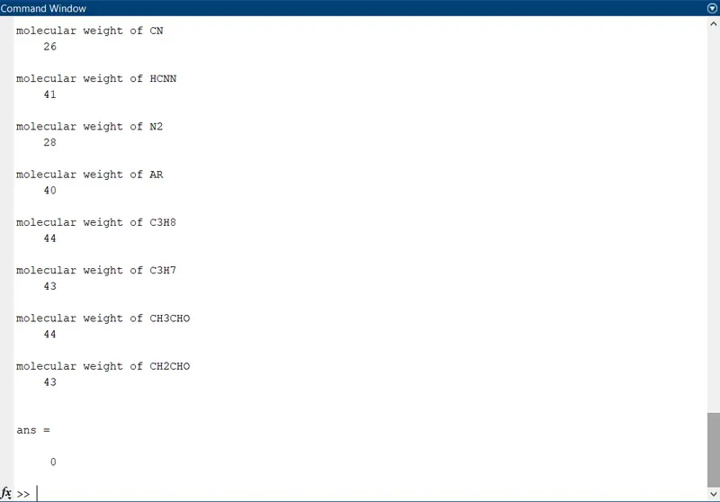
 disp(['molecular weight of ',species_name]);
 disp(Mw)
end

fclose(f1)
    

Explanation of the code –

To read the given Nasa file, fopen command is used and fgetl command is used to skip the line (i.e. to go to next line) First, the three lines of code (i.e. Header information) is read by strsplit command, which reads the individual strings by splitting the information with space between them. Str2num is used to convert strings to numbers.

From given data file, 53 species block are read using for loop, which will run 53 times to read species. The line is read by same strsplit command and given space to distinguish the information. Species name is given as first element as per the given data file.

To read the local temperatures of each and every species, flip command is used to easily read the line from end and then the elements are read by converting strings to numbers. Temperature is plotted from low local temperature to high local temperature with 500 parts using linspace command.

Then to read the coefficients, findstr command is used, by which Exponential (E) is located in each coefficient. With reference to that exponential, high temp and low temp coefficients are plotted as given in the problem. Then the functions of enthalpy, entropy, specific heat and molecular weight called in the main program and graph of temp vs enthalpy, entropy and specific heat are plotted for each species. By calling molecular weight, molecular weight of each element is displayed in the command window.

Function to plot the Enthalpy –

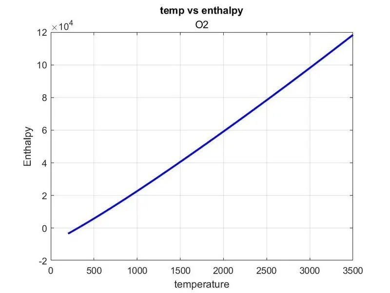
Function formula for enthalpy given in the problem is given as,

%Function to plot Enthalpy

% H/RT= a1+a2* T/2+a3 *T^2/3+a4*T^3/4+a5*T^4+/5+a6/T

function[h]= enthalpy_file_pa(a1,a2,a3,a4,a5,a6,b1,b2,b3,b4,b5,b6,R,temp,local_mid_temp)
if temp<=local_mid_temp
    h=R*temp.*(b1+ (b2.*(temp./2))+(b3.*(((temp).^2)./3))+(b4.*(((temp).^3)./4))+(b5.*(((temp).^4)./5))+b6./temp);
else
    h=R*temp.*(a1+ (a2.*(temp./2))+(a3.*(((temp).^2./3)))+(a4.*(((temp).^3)./4))+(a5.*(((temp).^4./5)))+a6./temp);
end
end

Function to plot the Entropy –

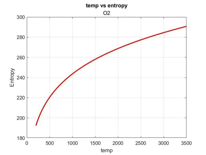
Function formula for entropy given in the problem is given as,

function[s]=entropy_file_pa(a1,a2,a3,a4,a5,a7,b1,b2,b3,b4,b5,b7,R,temp,local_mid_temp)
if temp<=local_mid_temp
s= R.*(b1.*log(temp)+(b2.*temp)+(b3.*(((temp).^2)./2))+(b4.*(((temp).^3)./3))+(b5.*(((temp).^4)./4))+b7);
else
s= R.*(a1.*log(temp)+(a2.*temp)+(a3.*(((temp).^2)./2))+(a4.*(((temp).^3)./3))+(a5.*(((temp).^4)./4))+a7);
end
end

Function to plot the Specific Heat –

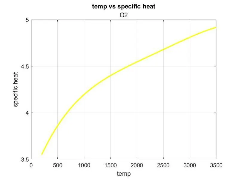
Function formula for specific heat given in the problem is given as,

%Function to plot the specific heat

%CP/R =a1+a2T+a3 T^2+a4 T^3+a5 T^4
function[c_p]=sp_heat_file_pa(a1,a2,a3,a4,a5,b1,b2,b3,b4,b5,temp,local_mid_temp)
if temp<=local_mid_temp
    c_p=(b1+ (b2.*temp)+(b3.*((temp).^2))+(b4.*((temp).^3))+(b5.*((temp).^4)));
else
    c_p=(a1+ (a2.*temp)+(a3.*((temp).^2))+(a4.*((temp).^3))+(a5.*((temp).^4)));
end
end

Function to plot the Molecular Weight –

%Function to plot the molecular Weight

function[Mw]=molecular_weight_file_pa(species_name)

elements=['H','C','N','O','A'];
atomic_weight=[1,12,14,16,40];

Mw=0;
for i=1:length(species_name)
    for j=1:length(elements)
        if strcmp(species_name(i),elements(j))
            Mw=Mw+atomic_weight(j);
            a=j;
        end
    end
    
n=str2double(species_name(i));
if n>1
    Mw=Mw+atomic_weight(a)*(n-1);
    
end
end
end

Explanation of the molecular weight code –

All the primary elements and their respective atomic weights are taken inside the program. Initially molecular weight is given as 0.

To get the molecular weight of the primary elements, for loops are used with species name and elements name. Both the conditions are verified by strcmp command. Mw is taken as initial Mw and atomic weight foe each and every element, so the molecular weight of the primary elements has been plotted.

In order to get the molecular weight of the species, n is given as numerical value for the concentration of each element. If condition is used when n is greater than 1, (i.e. concentration of one element is more in the given species for example. H2O) then molecular weight will get from the above formula as molecular weight of the first element plus the molecular weight of second element as per the list of elements from first to last and this is then multiplied by n-1 in order to get the actual weight. (For example Mw of O + Mw of H2*(2-1) will get the molecular weight of H2O)

Results –

Plots of O2

1. Temperature Vs Enthalpy -

2. Temperature Vs Entropy –

3. Temperature Vs Specific Heat

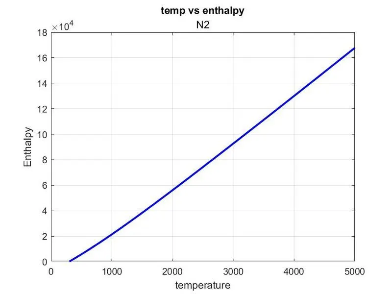
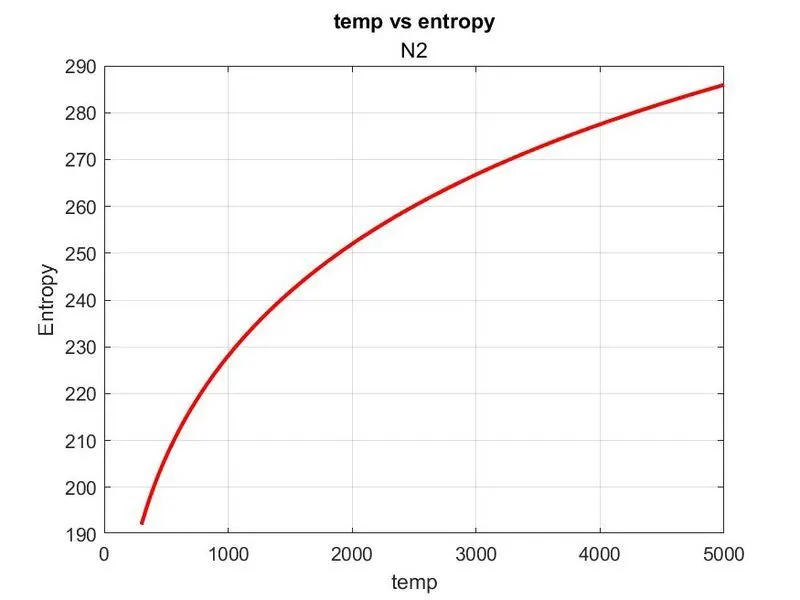
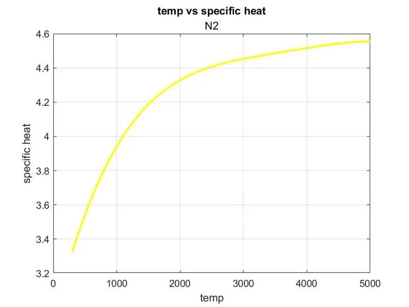
Plots of N2 –

1. Temperature Vs Enthalpy –

2. Temperature Vs Entropy -

3. Temperature Vs Specific Heat -

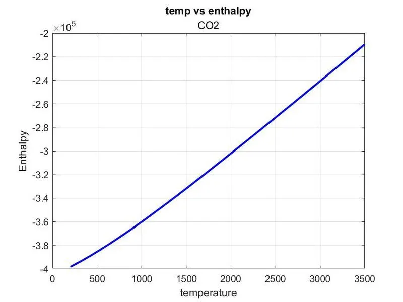
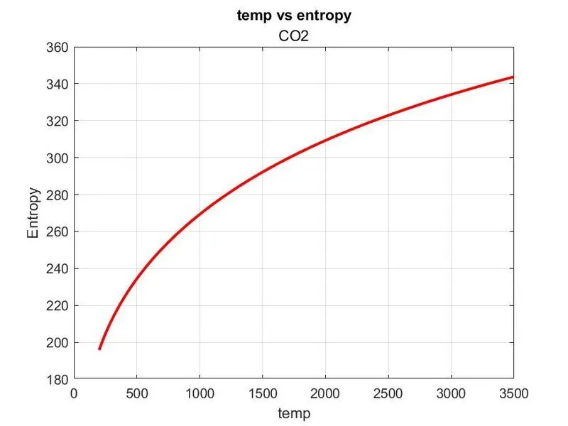
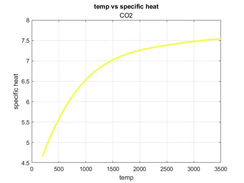
Plots of CO2 –

1. Temperature Vs Enthalpy –

2. Temperature Vs Entropy -

3. Temperature Vs Specific Heat -

Molecular Weight results –

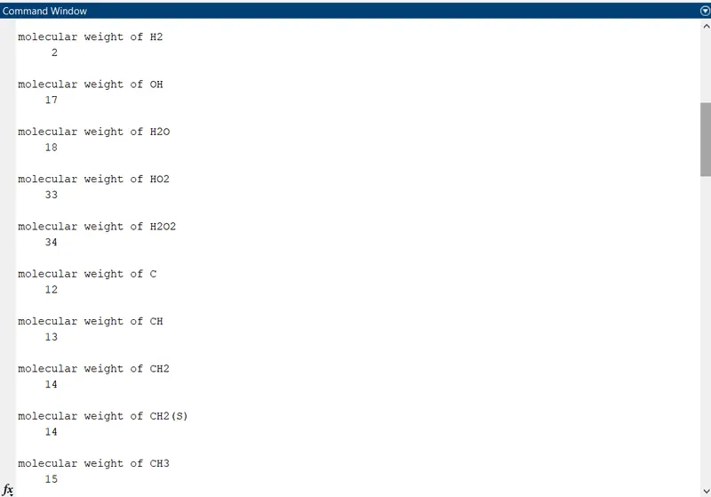
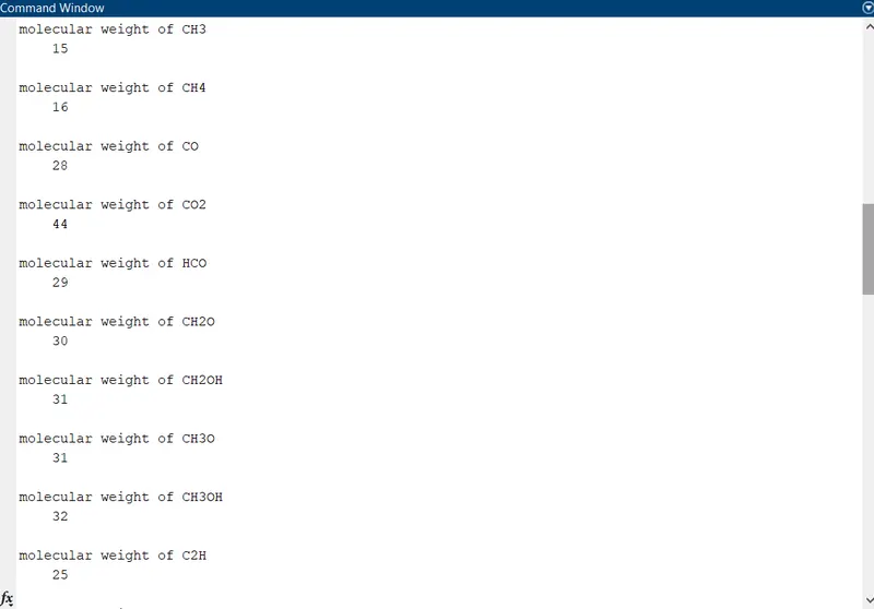
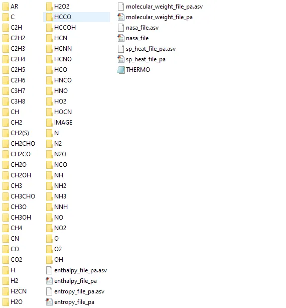
Screenshot of Nasa species folders -

CONCLUSION

Nasa theromodynamic data extarcted using matlab code and file parsing done sucesfully.