Week 8 - Simulation of a backward facing step in OpenFOAM
Simulation of backward facing step in openFoam
Objective :
- To simulate an incompressible-laminar-viscous flow through the backward facing step geometry and we should perform a transient simulation.
And we have to perform
-
Case 1 - Simulate the flow without using any grading factor (i.e., GF = 1)
Case 2 - Simulate the flow with grading factor of 0.2. The cells should be finer near the walls (includig the step wall).
- We have to measure the velocity profile at 0.085 m from the inlet of the geometry for both case studies and compare.
Theory :
Incompressible flow : In fluid dynamics, incompressible flow refers to a flow in which the density remains constant in any fluid parcel, i.e. any infinitesimal volume of fluid moving in the flow.
Laminar flow : Fluid (gas or liquid) flow in which the fluid travels smoothly or in regular paths .In laminar flow, sometimes called streamline flow, the velocity, pressure, and other flow properties at each point in the fluid remain constant. Laminar flow over a horizontal surface may be thought of as consisting of thin layers, or laminae, all parallel to each other. The fluid in contact with the horizontal surface is stationary, but all the other layers slide over each other.
Reynolds number is used to differentiate the flow between laminar and turblent.For flow in a pipe of diameter D, experimental observations show that laminar flow occurs when ReD < 2300 and turbulent flow occurs when ReD > 2900.
Viscous Flow : The fluid flow in which frictional effects become signification, are treated as viscous flow. When two fluid layers move relatively to each other, frictional force develops between them which is quantified by the fluid property 'viscosity'. Boundary layer flows are the example of viscous flow.
The flow which contains all these effects is called incompressible -laminar -viscous flow.
Solution procedure :
- Choosing a solver : The solver which suits for problem is icoFoam, which solves the incompressible laminar Navier-Stokes equations using the PISO algorithm.
- Selecting a solver tutorial : Here we choose the tutorial cavity from the incompressible icoFoam and we have to modify the geometry to a backward step in the blockmeshdict file.
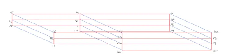
- The above is the geometry of backward step which is to be created by editing the blockmeshdict file.
The below are final modified files of blockmeshDict ,controlDict, pressure and velocity respectively.
blockmeshDict file :
/*--------------------------------*- C++ -*----------------------------------*\
  =========                 |
  \\      /  F ield         | OpenFOAM: The Open Source CFD Toolbox
   \\    /   O peration     | Website:  https://openfoam.org
    \\  /    A nd           | Version:  8
     \\/     M anipulation  |
\*---------------------------------------------------------------------------*/
FoamFile
{
    version     2.0;
    format      ascii;
    class       dictionary;
    object      blockMeshDict;
}
// * * * * * * * * * * * * * * * * * * * * * * * * * * * * * * * * * * * * * //


   convertToMeters 1;

vertices
(
    (0 0 0)
    (0.08 0 0)
    (0.08 0.005 0)
    (0 0.005 0)
    (0.08 0.01 0)
    (0 0.01 0)
    (0.2 0.01 0)
    (0.2 0.005 0)
    (0.2 0 0)
    (0.2 -0.01 0)
    (0.08 -0.01 0)
    (0 0 0.001)
    (0.08 0 0.001)
    (0.08 0.005 0.001)
    (0 0.005 0.001)
    (0.08 0.01 0.001)
    (0 0.01 0.001)
    (0.2 0.01 0.001)
    (0.2 0.005 0.001)
    (0.2 0 0.001)
    (0.2 -0.01 0.001)
    (0.08 -0.01 0.001)
);

blocks
(
    hex (0 1 2 3 11 12 13 14) (200 20 1) simpleGrading (1 1 1)
    hex (3 2 4 5 14 13 15 16) (200 20 1) simpleGrading (1 1 1)
    hex (10 9 8 1 21 20 19 12) (200 20 1) simpleGrading (1 1 1)
    hex (1 8 7 2 12 19 18 13) (200 20 1) simpleGrading (1 1 1)
    hex (2 7 6 4 13 18 17 15) (200 20 1) simpleGrading (1 1 1)

);

edges
(
);

boundary
(
   inlet
    {
        type patch;
        faces
        (
            (3 14 16 5)
            (0 11 14 3)
        );
    }
    outlet
    {
        type patch;
        faces
        (
            (20 9 8 19)
            (19 8 7 18)
            (18 7 6 17)
        );
    }
    frontAndBack
    {
        type empty;
        faces
        (
            (15 16 14 13)
            (13 14 11 12)
            (17 15 13 18)
            (18 13 12 19)
            (19 12 21 20)
            (5 4 2 3)
            (3 2 1 0)
            (4 6 7 2)
            (2 7 8 1)
            (1 8 9 10)
        );
    }
    noslipwalls
    {
    type  wall;
    faces
    (
               (4 5 16 15)
               (6 4 15 17)
               (0 1 12 11)
              (10 9 20 21)
              (1 10 21 12)
    );
    }
  );

mergePatchPairs
(
);


// ************************************************************************* //
controlDict file :
/*--------------------------------*- C++ -*----------------------------------*\
  =========                 |
  \\      /  F ield         | OpenFOAM: The Open Source CFD Toolbox
   \\    /   O peration     | Website:  https://openfoam.org
    \\  /    A nd           | Version:  8
     \\/     M anipulation  |
\*---------------------------------------------------------------------------*/
FoamFile
{
    version     2.0;
    format      ascii;
    class       dictionary;
    location    "system";
    object      controlDict;
}
// * * * * * * * * * * * * * * * * * * * * * * * * * * * * * * * * * * * * * //

application     icoFoam;

startFrom       startTime;

startTime       0;

stopAt          endTime;

endTime         0.3;

deltaT          0.00001;

writeControl    timeStep;

writeInterval   2000;

purgeWrite      0;

writeFormat     ascii;

writePrecision  6;

writeCompression off;

timeFormat      general;

timePrecision   6;

runTimeModifiable true;


// ************************************************************************* //
pressure file :
/*--------------------------------*- C++ -*----------------------------------*\
  =========                 |
  \\      /  F ield         | OpenFOAM: The Open Source CFD Toolbox
   \\    /   O peration     | Website:  https://openfoam.org
    \\  /    A nd           | Version:  8
     \\/     M anipulation  |
\*---------------------------------------------------------------------------*/
FoamFile
{
    version     2.0;
    format      ascii;
    class       volScalarField;
    object      p;
}
// * * * * * * * * * * * * * * * * * * * * * * * * * * * * * * * * * * * * * //

dimensions      [0 2 -2 0 0 0 0];

internalField   uniform 0;

boundaryField
{
    inlet
    {
        type            zeroGradient;
    }

    outlet
    {
        type            fixedValue;
        value            uniform 0;
    }

    frontAndBack
    {
        type            empty;
    }
    noslipwalls
    {
        type            zeroGradient;
    }
}
// ************************************************************************* //
velocity file :
/*--------------------------------*- C++ -*----------------------------------*\
  =========                 |
  \\      /  F ield         | OpenFOAM: The Open Source CFD Toolbox
   \\    /   O peration     | Website:  https://openfoam.org
    \\  /    A nd           | Version:  8
     \\/     M anipulation  |
\*---------------------------------------------------------------------------*/
FoamFile
{
    version     2.0;
    format      ascii;
    class       volVectorField;
    object      U;
}
// * * * * * * * * * * * * * * * * * * * * * * * * * * * * * * * * * * * * * //

dimensions      [0 1 -1 0 0 0 0];

internalField   uniform (0 0 0);

boundaryField
{
    inlet
    {
        type            fixedValue;
        value           uniform (1 0 0);
    }

    outlet
    {
        type            zeroGradient;
    }

    frontAndBack
    {
        type            empty;
    }
    noslipwalls
    {
        type            noSlip;
    }
}

// ************************************************************************* //
Post processing and plotting the results :After meshing by using blockMesh and running the case with icoFoam solver the next thing to do is to post process the results by using paraFoam in paraview and plotting the results by using plotover line command.
Case 1 - Simulating the flow without using any grading factor (i.e., GF = 1)
Mesh generated :
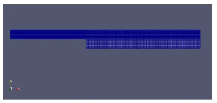
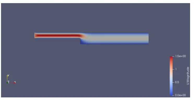
Velocity distribution along the geometry area :
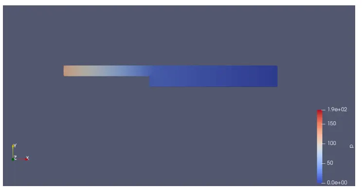
Pressure distribution along the geometry area :
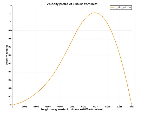
Velocity plot : The below plot is the velocity distribution ,Length along Y-axis at a distance of 0.085m from the inlet.
Case 2 - Simulating the flow with grading factor of 0.2.with cells finer near the walls .
To simulate the flow with simple grading with grading factor 0.2 we have to modify the blockMeshDict file.
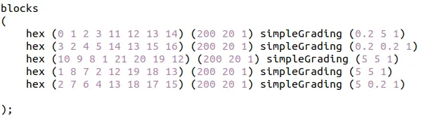
After the grading ,now run the blockMesh and then run solver icoFoam .The next thing to do is to post process the results by using paraFoam in paraview and plotting the results by using plotover line command.
Mesh generated :
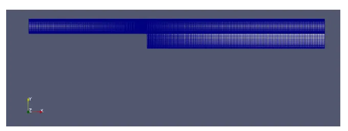
Velocity distribution along the geometry area :
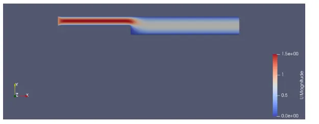
Pressure distribution along the geometry area :
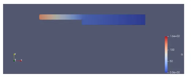
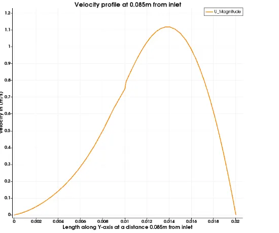
Velocity plot : The below plot is the velocity distribution ,Length along Y-axis at a distance of 0.085m from the inlet, captured with grading factor 0.2.
:
Now finally we can conclude that by seeing the plots, when we use the grading factor and refined the mesh we can see that the flow is captured exactly than without grading factor.At a distance 0.01 along Y-axis from a distance 0.085m from the inlet we can see that the flow is captured exactly that there is a sharp rise in value of velocity which was not captured well before.So using the finer mesh will lead to accurate results but it costs a lot of computational effort.