Week 9 - FVM Literature Review

Objective:

To study and understand

1. what is the Finite volume method(FVM)?.

2. The differnce between FDM and FVM.

3. Interpolation schemes in FVM.

4. Flux limiters in FVM.

1.What is Finite Volume Method(FVM) ?

The Finite Volume Method (FVM) is a numerical technique used to solve partial differential equations (PDEs) by discretizing the domain into control volumes and approximating the behavior of the solution at the volume averages. It is widely used in computational fluid dynamics (CFD), heat transfer analysis, and other fields involving conservation laws.

In FVM, the domain is divided into a set of non-overlapping control volumes or cells. The governing equations, such as conservation laws, are integrated over each control volume to obtain a set of discrete equations. The values of the solution variables, such as fluid properties or temperature, are represented by the cell averages within each control volume.

The key idea of FVM is to approximate the fluxes across the control volume faces using numerical schemes. These fluxes represent the net flow of the conserved quantities, such as mass, momentum, or energy, into or out of each control volume. The fluxes are computed based on the values of the solution variables at the cell interfaces using interpolation and gradient calculation schemes.

The discretized equations for each control volume are typically expressed in the integral form, where the fluxes across the control volume faces are integrated over the corresponding faces. These equations can be solved iteratively or using time-stepping methods to obtain the time-dependent or steady-state solution.

FVM has several advantages that make it popular in many engineering applications. It naturally conserves quantities within control volumes, ensuring accurate representation of global conservation laws. FVM can handle complex geometries, irregular meshes, and unstructured grids, making it versatile for simulating a wide range of physical systems. It also provides good control over numerical diffusion and allows for accurate capture of discontinuities, such as shocks or sharp gradients.

Overall, FVM is a powerful numerical method for solving PDEs by discretizing the domain into control volumes and approximating the fluxes across control volume faces. It provides an effective approach to simulate various physical phenomena and is widely used in engineering and scientific simulations.

2. The differnce between FDM and FVM.

2.1 Finite Volume Method (FVM):

1. Control Volume Approach: FVM treats the computational domain as a collection of control volumes. Each control volume is a discrete region of space where the governing equations are integrated. The control volumes can be of different shapes and sizes and are typically defined by the mesh or grid. The method focuses on the conservation of fluxes across control volume faces, ensuring that the integral form of the governing equations is satisfied.

2. Flux Calculation: FVM approximates the fluxes across the control volume faces by considering the average values of the variables inside each control volume. The fluxes are typically calculated using numerical schemes such as upwind schemes, central differencing, or higher-order schemes. The choice of the scheme depends on the nature of the problem being solved.

3. Conservation of Quantities: FVM inherently conserves quantities such as mass, momentum, and energy due to its integral formulation. This conservation property makes it suitable for solving problems governed by conservation laws. By ensuring that the fluxes are properly accounted for across control volume faces, FVM provides accurate results for the average values of the variables within each control volume.

2.2 Finite Difference Method (FDM):

1. Grid Point Approach: FDM discretizes the computational domain using a grid of points. The governing equations are approximated at these grid points, and the derivatives are calculated using finite differences. The choice of the grid spacing, also known as the mesh size or grid resolution, affects the accuracy of the solution.

2. Finite Difference Approximation: FDM approximates the derivatives in the governing equations using finite difference formulas. These formulas express the derivative at a grid point in terms of the function values at nearby grid points. Common finite difference schemes include forward difference, backward difference, and central difference schemes. The accuracy of the approximation depends on the order of the scheme.

3. Boundary Conditions: FDM often requires special treatments for imposing boundary conditions. Different techniques like ghost points, extrapolation, or modification of the difference formulas are used to ensure that the boundary conditions are satisfied. The choice of boundary treatment can influence the accuracy and stability of the solution.

2.3 Table summarizing the key differences between the Finite Volume Method (FVM) and the Finite Difference Method (FDM):

Aspect	Finite Volume Method (FVM)	Finite Difference Method (FDM)
Discretization Approach	Control volume approach	Grid point approach
Conservation Property	Inherently conserves quantities	May require additional techniques
Grid Types	Handles irregular and non-uniform grids	Suited for regular grids
Treatment of Boundaries	Handles boundaries using control volume faces	Requires specific treatments or modifications
Flux Calculation	Approximates fluxes across control volume faces	Approximates derivatives at grid points
Interpolation Schemes	Not typically required	May be used for higher-order accuracy
Flux Limiters	Used to control numerical oscillations and maintain stability	Not commonly used
Accuracy and Convergence	Can achieve higher-order accuracy with appropriate schemes	Typically lower-order accuracy
Computational Efficiency	Requires more computational resources due to larger number of control volumes	Generally more computationally efficient with smaller stencil
Handling Irregular Domains	Adaptable to irregular domain shapes and complex geometries	May require special treatments for irregular domains
Robustness	Tends to handle discontinuities and shocks better	May suffer from numerical instability and spurious oscillations
Implementation Complexity	Moderate complexity due to control volume integration	Simpler implementation with finite difference formulas
Application Range	Suitable for conservation laws and flow problems	Widely applicable to various types of PDEs

3. Interpolation schemes in FVM.

Interpolation Schemes: Interpolation schemes are necessary in FVM to estimate the values of variables at the control volume faces or cell interfaces. They ensure accurate representation of the variables at the face locations, which are essential for calculating the fluxes across the control volume faces. Here are some commonly used interpolation schemes:

a. Piecewise Constant (Zeroth-Order) Scheme: This is the simplest interpolation scheme, where the variable is assumed to be constant within each control volume. The value at the face is taken as the value inside the control volume, providing a piecewise constant approximation.

b. Linear (First-Order) Scheme: The linear interpolation scheme assumes a linear variation of the variable within each control volume. It uses the values at the adjacent cell centers to estimate the value at the face. The linear scheme provides a piecewise linear approximation.

c. Higher-Order Polynomial Schemes: These schemes utilize higher-order polynomial interpolations to improve the accuracy of the approximation. Examples include the quadratic scheme (second-order), cubic scheme (third-order), and so on. These schemes provide smoother representations and better accuracy but come with increased computational complexity.

Need for Interpolation schemes

1. In Finite volume method (FVM), the flow variables are stored in the centroid (P, N) of the cell as shown in the figure below.
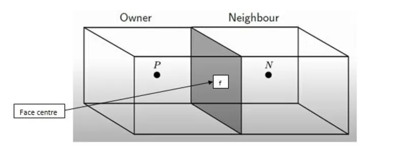
2. The navier stokes equation is integrated across the cell volume i.e., volume integrals are solved for each cell. The navier stokes equation normally contains convection term, pressure gradient, diffusion term and a source term.
3. For solving the convection & diffusion terms, the gauss divergence theorem is used and the volume integrals are converted into surface integrals.
4. Each cell can have numbers of faces depending on the type of mesh and each face will be associated with a neighbouring cell. The velocities at centre of each face of the corresponding cell are computed.
5. In order to compute the face centre velocity the interpolation in needed as the face centre velocity is calculated using velocity at the owner and neighbour cell centroids.
6. In setting up a CFD code - discretization is a very basic and while choosing the discretization schemes we are actually choosing an interpolation method.
7. There are different interpolation schemes available such as Upwind, Linear upwind, Central Differencing, and QUICK.
8. These schemes calculate the face centre values using information at the owner and neighbour cell centroids.

4.Flux limiter in FVM:

For convective fluid flow, it is ovservedthat low order schemes are usually stable but quite dissipative in nature around the points of discontinuity or shocks while the higher order schemes are unstable in nature and show oscillations in the vicinity of dinscontinuity or shocks. Highly accurate and oscillation free schemes are known as High Resolution Schemes.

In order to make the scheme TVD, we must constrain or limit the range of possible values of the additional convective flux , which was originally introduced to make the scheme higher-order. Hence, the function is called a flux limiter function.

Flux Limiter functions are used to fine tune the higher order and lower order schemes in such a way that the resulting scheme gives a higher order accuracy in the smooth region of the flow and maintains first order accuracy in the vicinity of shocks and discontinuities. For such a scheme TVD scheme is employed.

1. Flux limiter is a mechanism to address the source of oscillation especially the non-physical oscillation in an extrapolation.
2. Extrapolation is good in a smooth region but it’s bad especially near the near discontinuities.
3. As the FVM deals with the cell averages, if the cell average of current cell is greater or less than its left or right neighbouring cell’s average then the sudden oscillation will occur due to the local maxima and minima.
4. So flux limiter detects such situation i.e., the local maxima or minima then turns off the extrapolation from one cell to another and goes back to piece wise constant approximation.
5. But if the cell averages of current and neighbouring cells are almost the same then extrapolation is used.
6. It’s basically a switch as it switches between extrapolation and piece wise constant approximation depending on the situation. So for a smooth switching and continuous solution from one cell to another flux limiters are very crucial.

Conlusion:

Finite Volume Method (FVM) is really a powerful approach to solve the CFD problems. With the help of proper interpolation schemes and the accurate use of flux limiters in case of any discontinuities present, we can solve a wide range of CFD problems.

Though it may be difficult to code and implement it in the computer it gives an added advantage of its robustness