Week 3 - External flow simulation over an Ahmed body.

Q1. Ahmed body is a benchmark for validating simulation tool. As we all know major factor in validating any car model is its aerodynamic efficiency. If a car is aerodynamically efficient i.e., less drag is generated by the car, its fuel efficiency will also increase. But for complex car model it is difficult to validate the result computationally. So, for that purpose Ahmed body is used to validate the simulation tool.

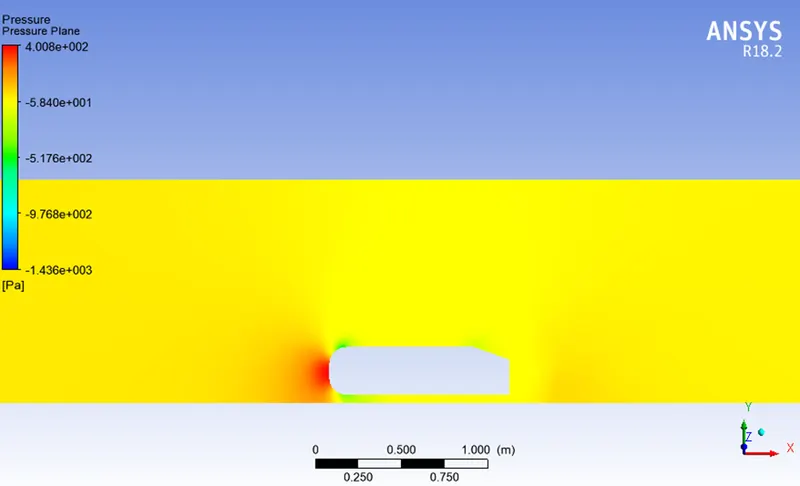
Q2. If we follow the path of the fluid, we can clearly understand the reason of negative pressure in the wake region. So, we the fluid comes in contact with the Ahmed body, the flow accelerates and the pressure gradient decreases, but as the flow continues the flow decelerates and pressure gradient begins to increase, this is called adverse pressure gradient. Due to increase in pressure fluid wants to travel back to low pressure area i.e., in reverse direction, but due to oncoming fluid it detaches itself from the boundary layer and starts recirculating. Because of the detachment of fluid at the rear end of the car, a negative pressure is created in the wake region.

Q3. The point at which the pressure gradient increases and fluid detaches it self from boundary layer is called point of separation. For Laminar flow, the point of separation is early than the turbulent flow. If the point of separation is early then the low-pressure wake region created will be big which will lead to increase in Pressure drag. So, if the point of separation is late, lower is the pressure drag. So, in many cases to create turbulence, vortex generators are placed to make flow turbulent and in doing so decrease the drag.

Baseline Model approach:

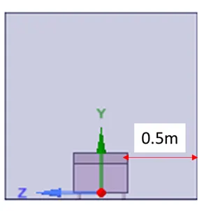
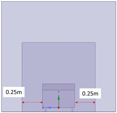
1. First, we will load the model in space claim and create enclosure with below dimension.

2. Now Geometry is loaded for Meshing where we will give default meshing with mesh length of 412.3 mm. Number of Mesh elements: 84836.

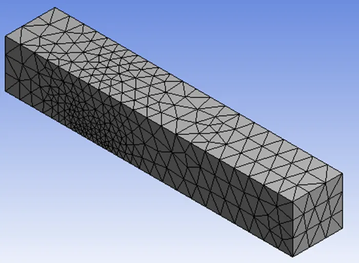
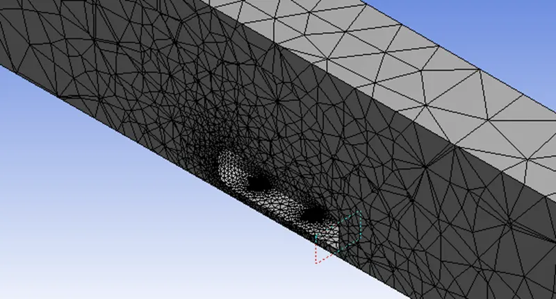
3. Once the meshing is done, we will setup the physics for solving the baseline of Ahmed body and based on the result we will do refining.

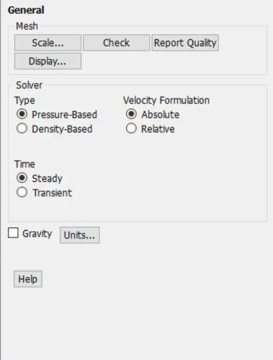
a. We will use pressure-based solver as the speed of inlet will be 25 m/s i.e., 0.072 Mach which is less than 0.3. General rule that is followed is when Mach is greater than 0.3, we should consider compressibility of the fluid as well and for that Density-based solver is used. But, in our case as Mach is less than 0.3, we can use pressure-based solver.

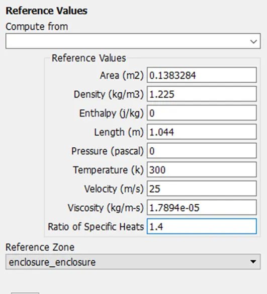
b. Reference Values

Frontal Area of Ahmed Body:

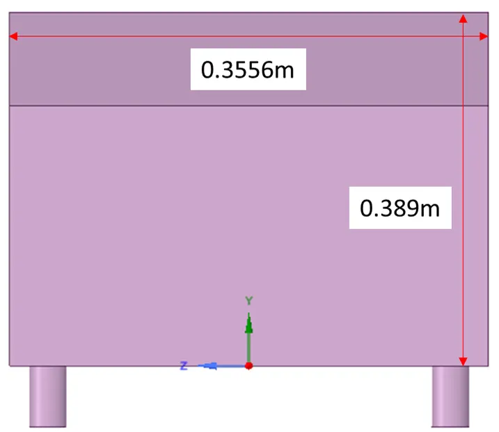
Area = 0389*0.3556 = 0.1383284 m^2

Length of Ahmed Body:

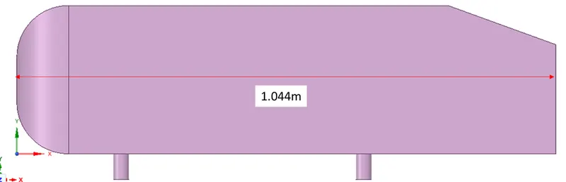
Characteristics length of the flow = 1.044 m

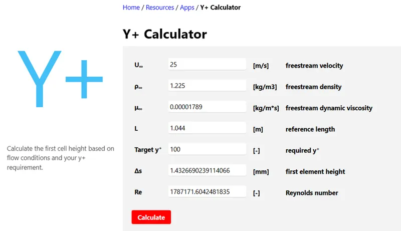
Reynolds Number = `(rho*V*L)/mu` = `(1.225*25*1.044)/(1.7894*e^-5)`= 1.787 e6

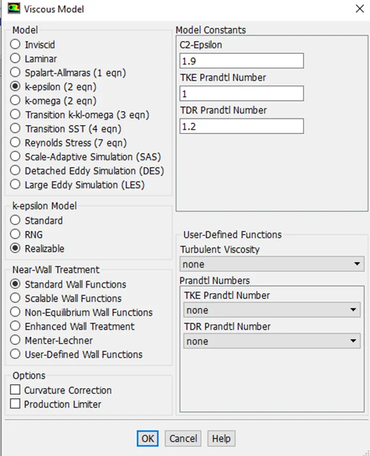
So, as Reynold’s number is in turbulent regime we will use K-epsilon model for initial analysis and based on the results we can decide weather to stick with K-epsilon or to change the solver model.

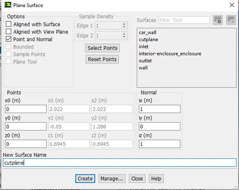
c. We will also create a cut plane such that it passes through the centre of Ahmed body, so that we can view contours of pressure and velocity around the Ahmed Body.

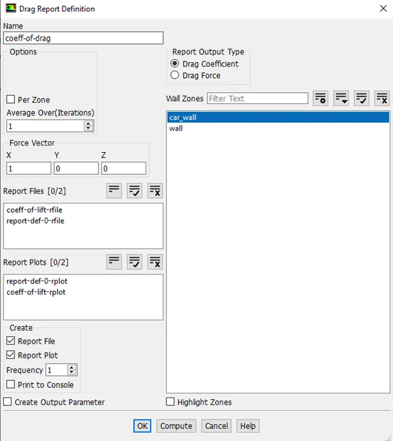
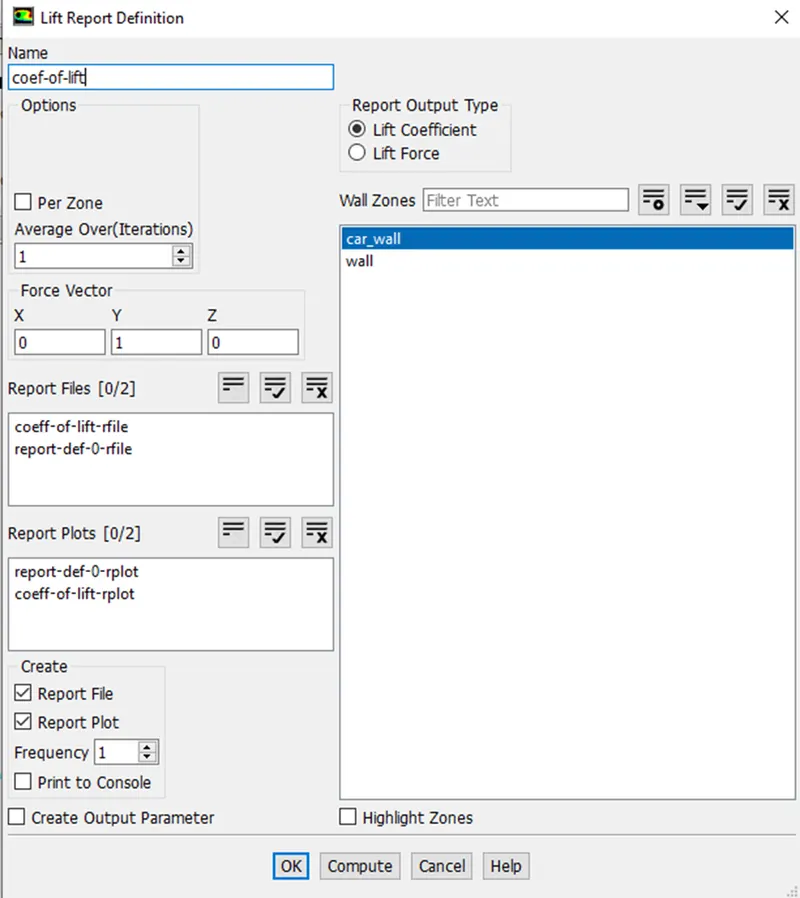
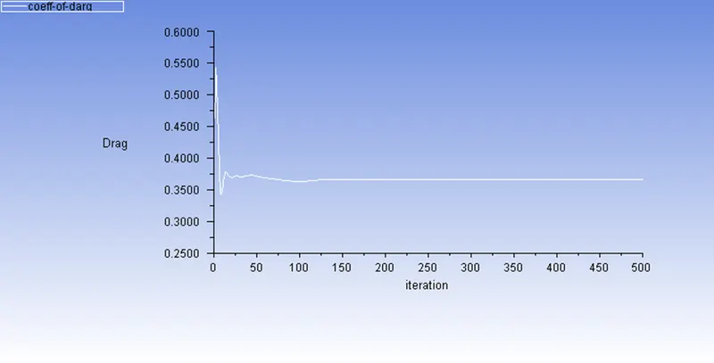
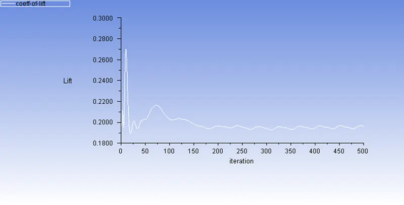
d. We will also create reports of Coeff-of-Drag and Coeff-of Lift as the result is being computed.

e. Now we can initialize the solution using Hybrid method as it will provide a good initial result.

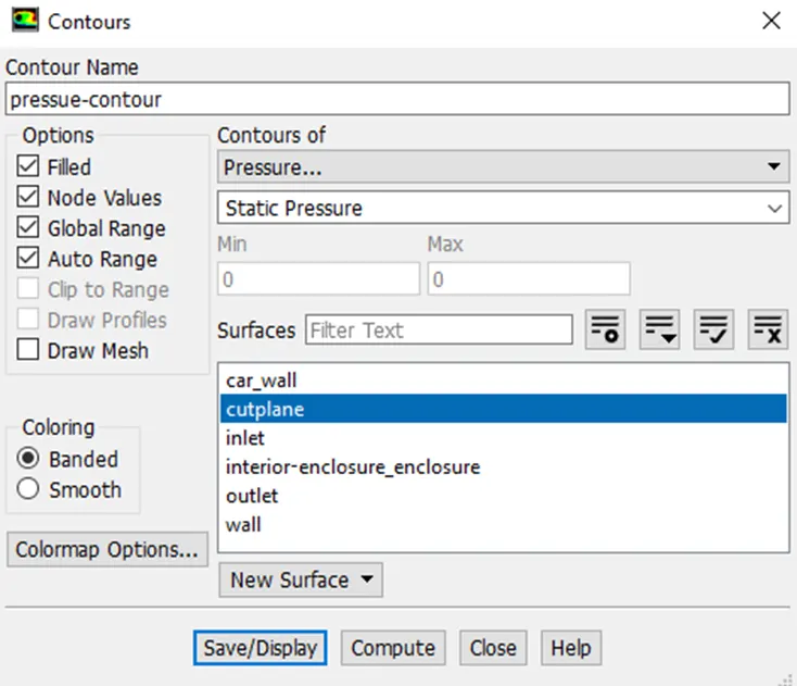
f. Once the solution is initialized, we can setup contours for pressure and velocity at cut plane.

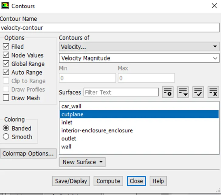
4. Now we will, run the simulation till we get a converged result

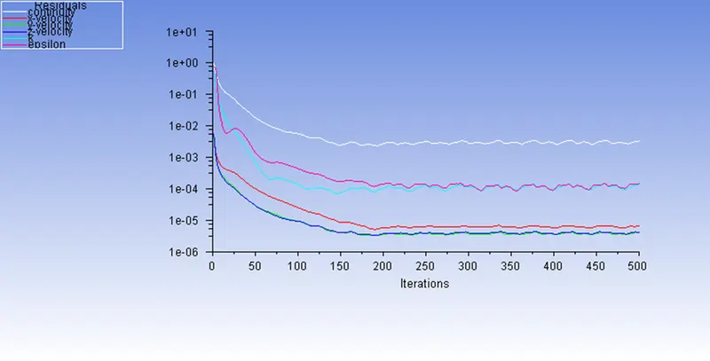
At 500 iterations we see that the residual is forming same pattern. So, we can say that the solution is converged.

a. Coeff of Drag: 0.3667

b. Coeff of Lift: 0.1964

c. Pressure Contour:

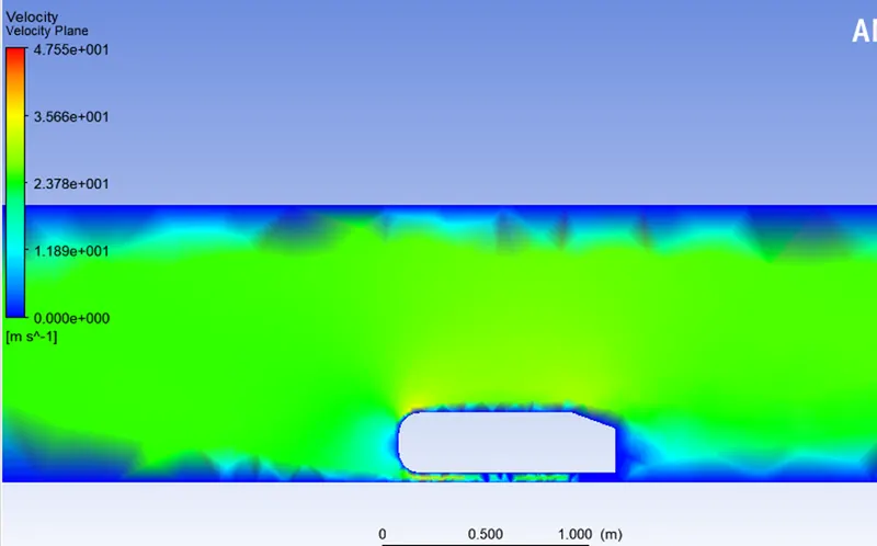
d. Velocity Contour:

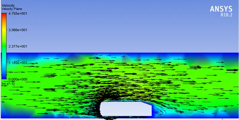
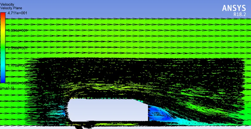
e. Vector Plot:

5. As we see from above results, the solution near the wall of the car is very coarse and is not showing a refined solution. So, mesh refinement is a must for the above case. As we are looking at the solution near wall its better to K-omega turbulent model.

Refinement Model-1

1. For refinement of the model, we could introduce another enclosure within with a very refined mesh compared to what we had in previous case. This will be effective as it will prevent number of elements increasing drastically in name of mesh refinement.

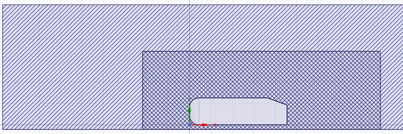
2. To introduce another enclosure, we need to open space claim and create another enclosure for the Ahmed body, but with a smaller size.

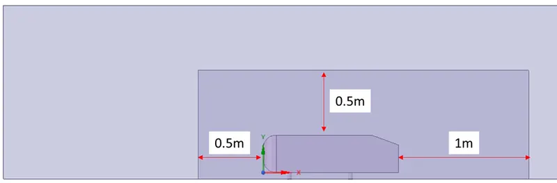
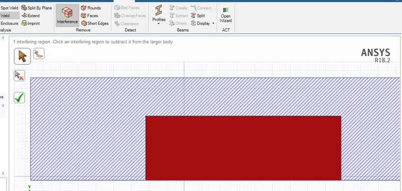
3. If we look at the section view, we can see that both the enclosures are interfering with each other, which could cause meshes to overlap each other. This will affect the mesh quality. So, we can remove overlapping models using Interference option in space claim.

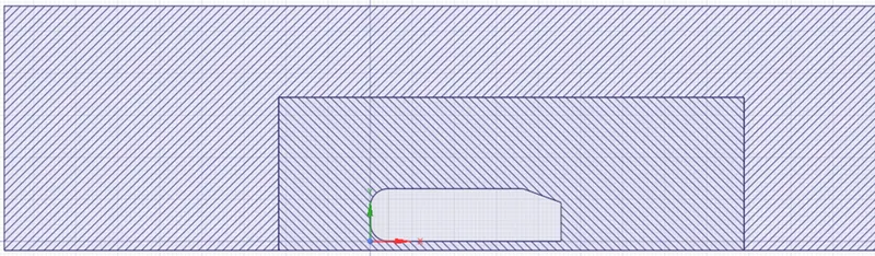4. Now we move on to meshing. In meshing, as the outer surface consist of only straight lines, we can create a hexadecimal meshing for the same. For that we have insert a method called multizone and we need to select outer body with Hexa as dominant mesh element.

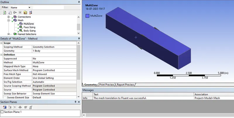
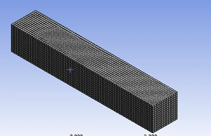
We have given maximum mesh length of 100 mm, So outer body looks like the below image

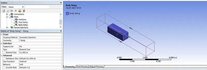
For inner enclosure, we have created sizing parameter of 50 mm as below

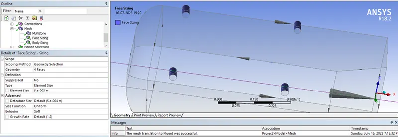
And for the pillars of Ahmed body, to retain its shape we have given a face sizing of 5 mm as below

We will also introduce inflation layer for mesh wall with first layer thickness of 5mm

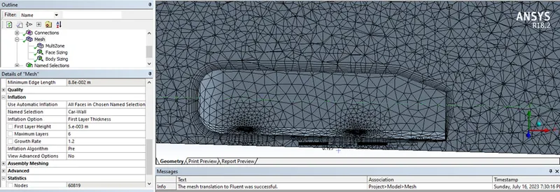
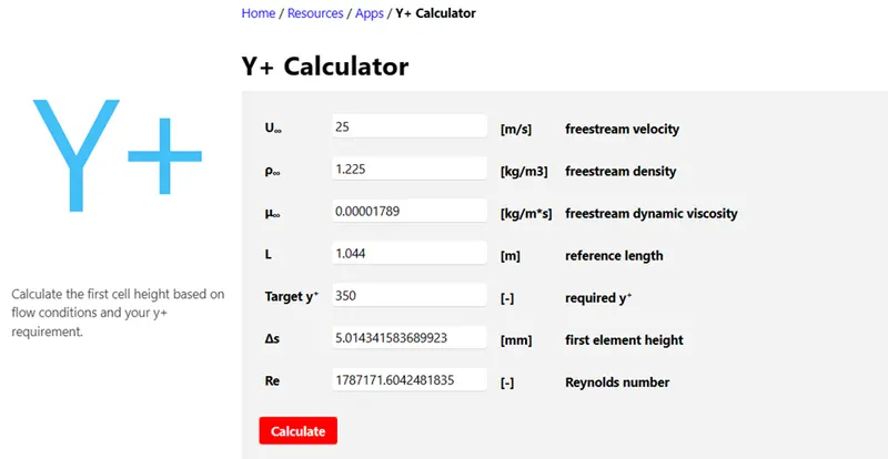
So, we get a y+ value of approx. 350 based on below calculator.

At the end of meshing, we have total of 188336 mesh elements present in the geometry

5. As, the meshes are now much more refined we can run the simulation with K-omega SST model.

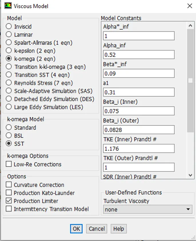
6. Now we will, run the simulation till we get a converged result

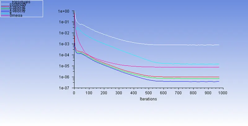
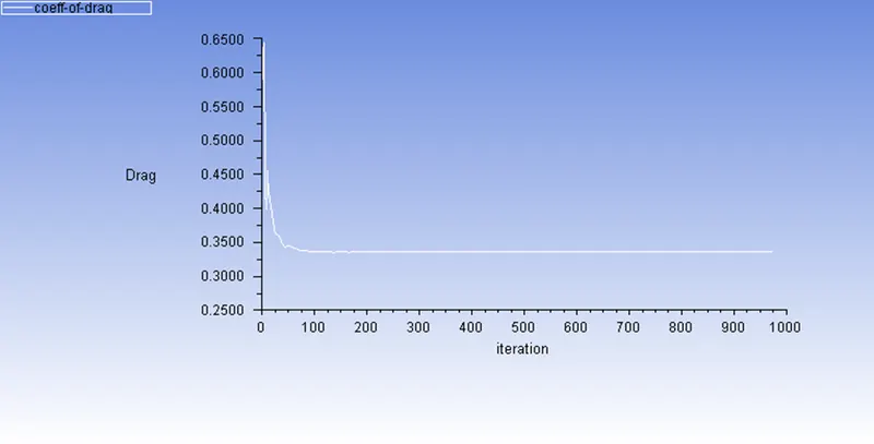
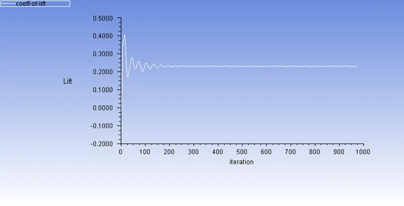
At 950 iterations we see that the residual is forming same pattern. So, we can say that the solution is converged.

a. Coeff of Drag: 0.3358

b. Coeff of Lift: 0.2325

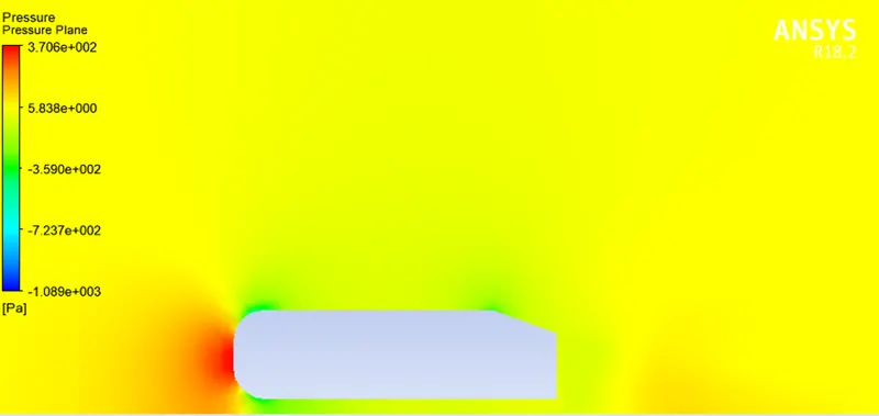
c. Pressure Contour:

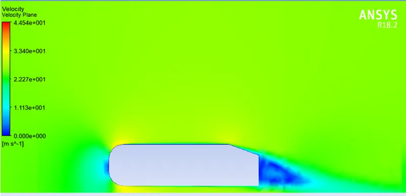
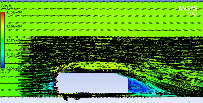
d. Velocity Contour:

e. Vector Plot:

Refinement Model-2:

1. For more refinement than previous case we have reduced the Mesh size to 90 mm for outer body, and 45 mm for inner body

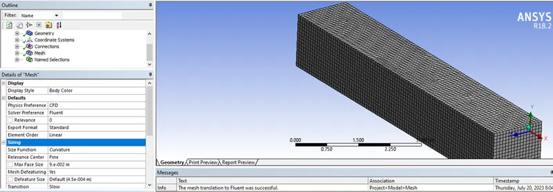
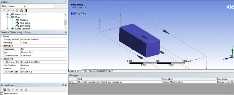
2. We have reduced the first layer height in inflation layers to 2.86 mm and increased number of inflation layer to 10.

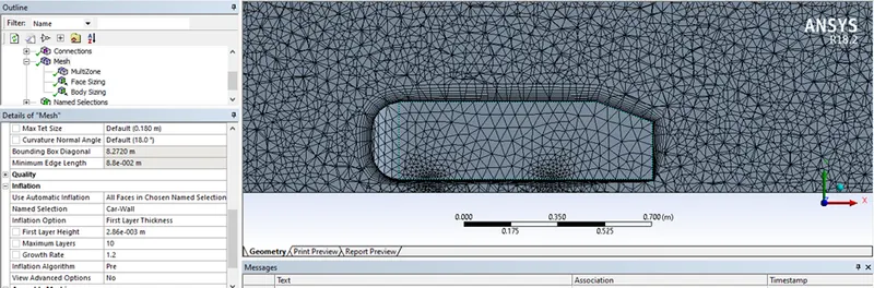
Based on the calculation shown below, we get a Y+ value of approx. 200

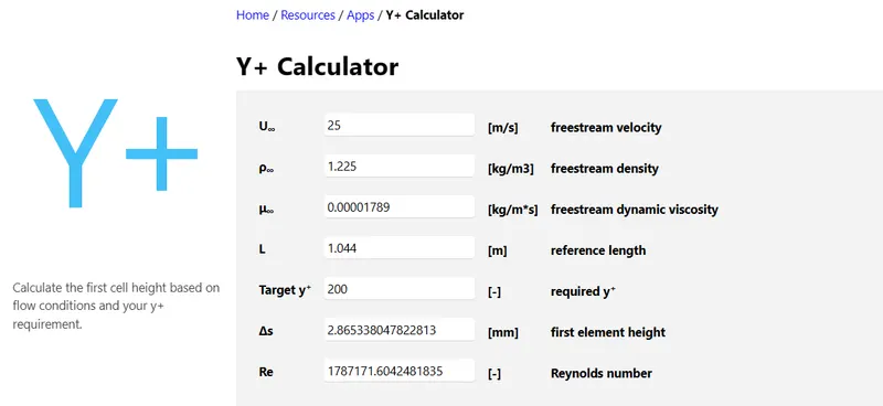
Total Mesh Elements: 258655

3. We don’t need to change setup for this case as we have only refined the meshes for calculating the results.

4. Now we will, run the simulation till we get a converged result

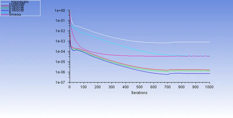
At 1000 iterations we see that the residual is forming same pattern. So, we can say that the solution is converged.

a. Coeff of Drag: 0.3247

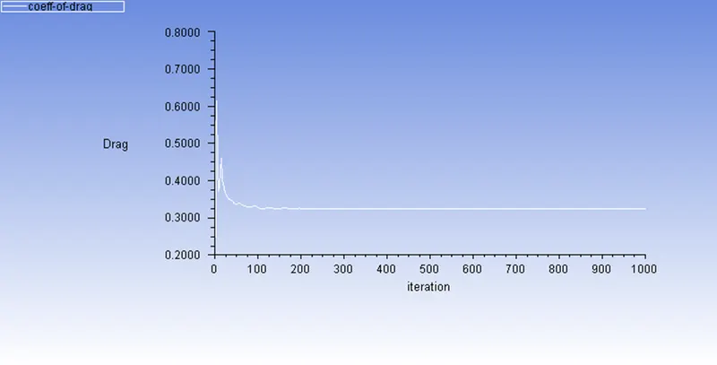
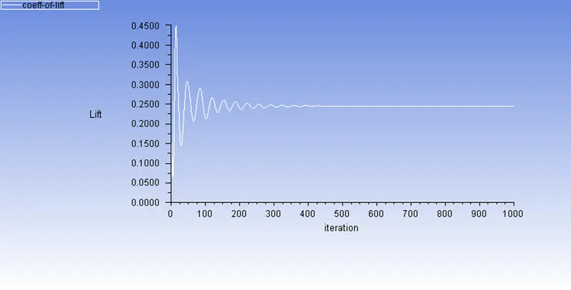
b. Coeff of Lift: 0.2450

c. Pressure Contour:

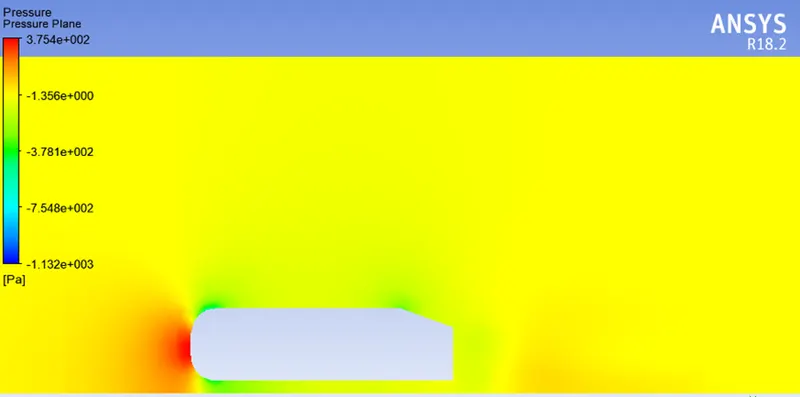
d. Velocity Contour:

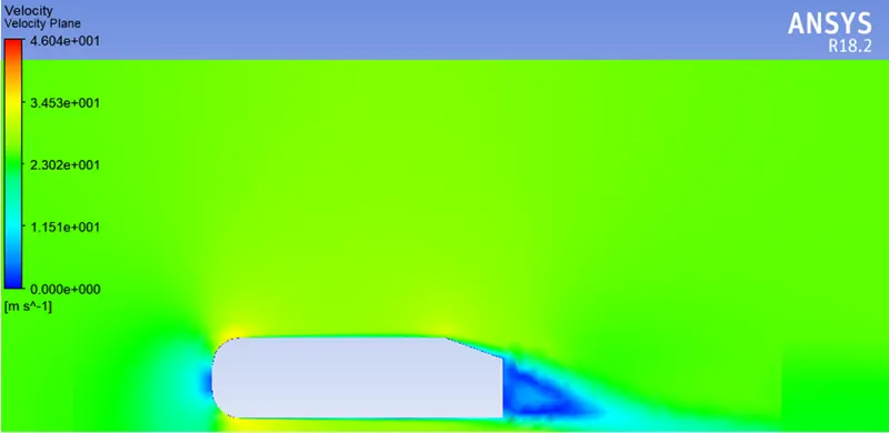
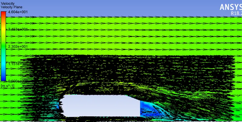
e. Vector Plot:

Refinement Model-3:

1. For more refinement than previous case we have reduced the Mesh size to 80 mm for outer body, and 40 mm for inner body.

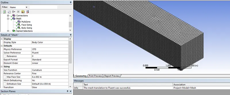
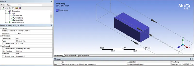
2. We have reduced the first layer height in inflation layers to 1.43 mm and increased number of inflation layer to 10.

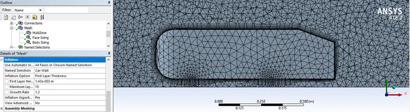
Based on the calculation shown below, we get a Y+ value of approx. 100

Total Mesh Elements: 342334

3. We don’t need to change setup for this case as we have only refined the meshes for calculating the results.

4. Now we will, run the simulation till we get a converged result

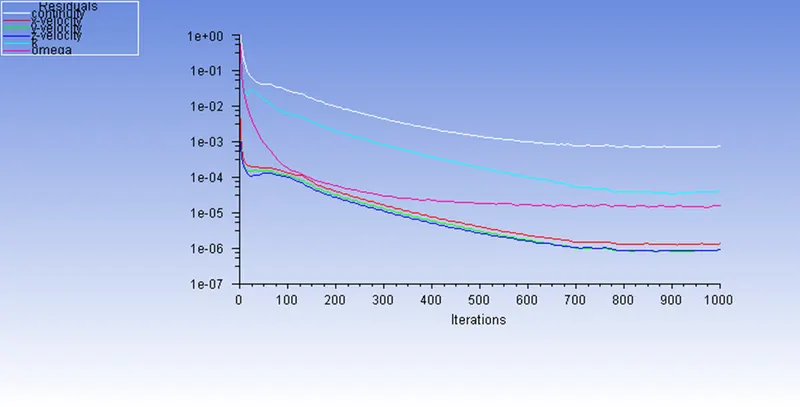
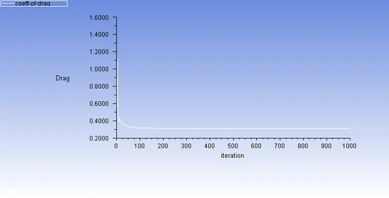
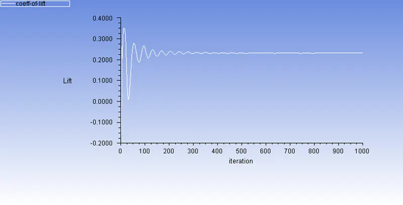
At 1000 iterations we see that the residual is forming same pattern. So, we can say that the solution is converged.

a. Coeff of Drag: 0.3200

b. Coeff of Lift: 0.2316

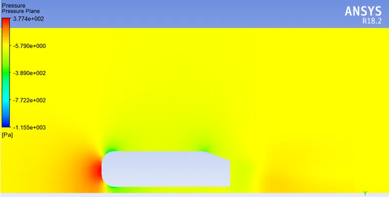
c. Pressure Contour:

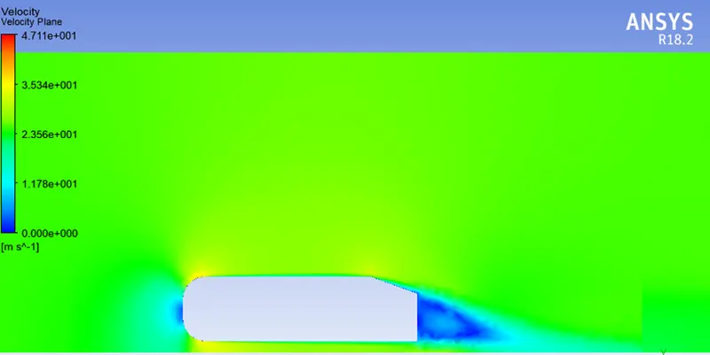
d. Velocity Contour:

e. Vector Plot:

Inference:

As we keep on reducing Mesh size, we observe that there is decrease in Drag, but after second refinement the decrease in coefficient of drag is negligible. So, we can concur that we can save time by using a smaller cell size for simulation.

Grid Independence	Turbulence Model	No. of Elements	Drag Coefficient
Baseline	K-epsilon Realizable	84836	0.3667
Refined model 1	K-Omega SST	188336	0.3358
Refined model 2	K-Omega SST	258655	0.3247
Refined model 3	K-Omega SST	342334	0.3200

Conclusion:

• A grid independence test was performed to check the cell size for the convergence of the solution.
• Apart from mesh refinement, the convergence of solution also depended on Y+ value, as the Y+ value was decreasing more accurate results were curated. Also, in this case, solution near wall was of utmost importance, so K-omega was used as it is better at giving solution near wall compared to K-epsilon.
• As cell size went on decreasing the Coefficient of drag and lift also decreased.
• A Negative pressure was created in the wake region of the car as, there is no flow of fluid there, which further attributed to recirculation which is evident from vector plot.
• The point of separation is at the rear end of vehicle, at the end point, and we can observe that beyond that point flow recirculates and attaches itself to boundary layer