Week 3 - External flow simulation over an Ahmed body.
EXTERNAL FLOW OVER AN AHMED BODY
AIM: To stimulate the external flow over an ahmed body for the different cases like coarse mesh and refined mesh.
OBJECTIVE:
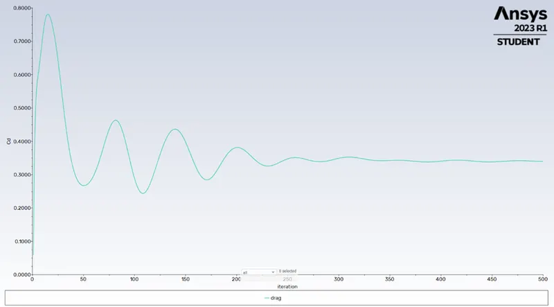
To attain the co-efficient of drag value around 0.33 for velocity of 25m/s with help of the grid independence test.
Expected results: -
- Velocity and pressure contours.
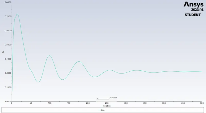
- The drag coefficient plot for a refined case. (For velocity of 25m/sec, the drag coefficient should be around 0.33).
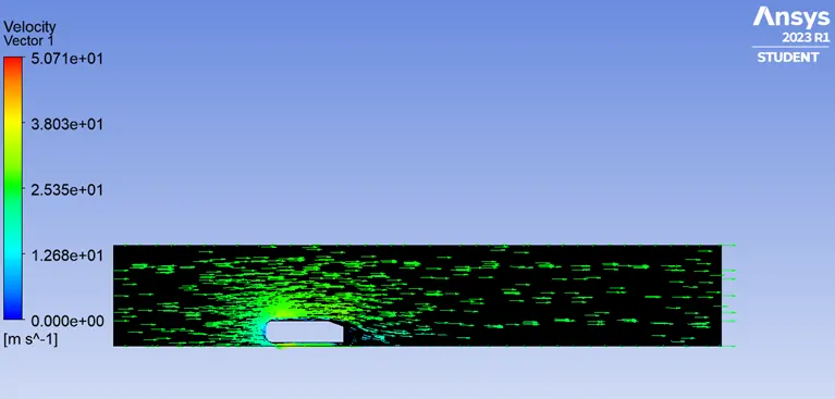
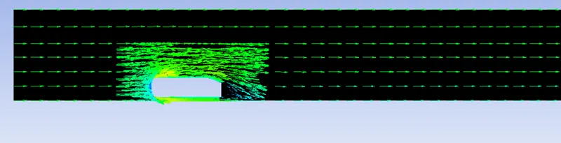
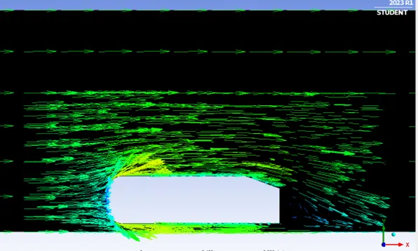
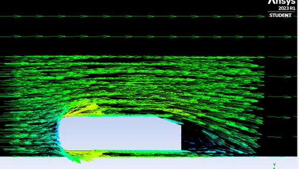
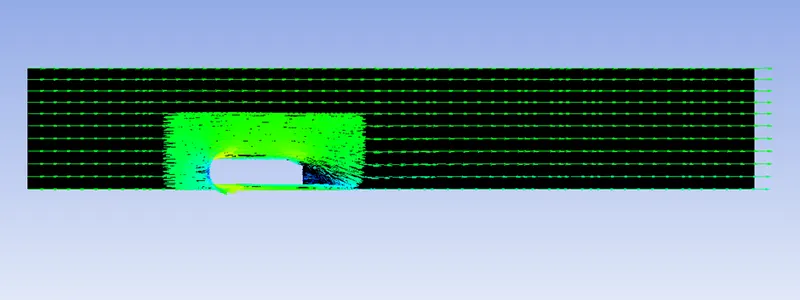
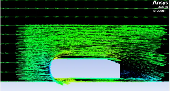
- The vector plot clearly showing the wake region.
- Perform the grid independency test and provide the values of drag and lift with each case.
INTRODUCTION:
The Ahmed Body was first created by S.R. Ahmed in his research “Some Salient Features of the Time-Averaged Ground Vehicle Wake” in 1984. Since then, it has become a benchmark for aerodynamic simulation tools. The simple geometrical shape has a length of 1.044 meters, height of 0.288 meters, and a width of 0.389 meters. It also has 0.5-meter cylindrical legs attached to the bottom of the body and the rear surface has a slant that falls off at 40 degrees.
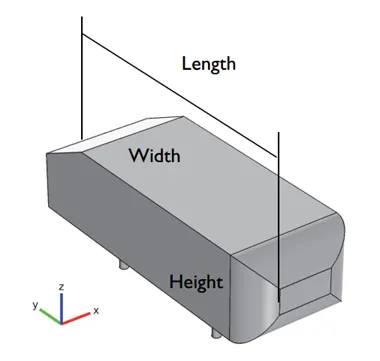
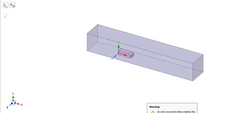
In the airflow over an ahmed verification model, our Ahmed body has a 25-degree slant and is placed in the following domain, measuring 8.352-by-2.088-by-2.088 meters, to compute the flow field.
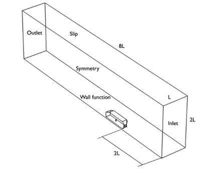
Computational domain and boundary conditions for the fluid flow simulation.
The front of the body is placed at distance of 2 car lengths (2L) from the flow inlet. To reduce the computational cost, a symmetry plane is introduced to model half of the model.
The flow for this model is turbulent, which is based on the Reynolds number determined by the body length and inlet velocity. The simulation solves for the turbulent kinetic energy in addition to the velocity field. For this simulation, we need a larger mesh size than what is usually common to resolve the turbulent flow. More specifically, we use a finer mesh downstream of the model to capture the wake zone.
The flow for this model is turbulent, which is based on the Reynolds number determined by the body length and inlet velocity. The simulation solves for the turbulent kinetic energy and dissipation in addition to the velocity and pressure fields.
Wake Region and Point of Separation:
Pressure gradient is an is one of the factors that influences a flow immensely. It is easy to see that the shear stress caused by viscosity has a retarding effect upon the flow. This effect can however be overcome if there is a negative pressure gradient offered to the flow. A negative pressure gradient is termed a Favourable pressure gradient. Such a gradient enables the flow. A positive pressure gradient has the opposite effect and is termed the Adverse Pressure Gradient. Fluid might find it difficult to negotiate an adverse pressure gradient. Sometimes, we say the fluid must climb the pressure hill.
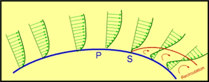
One of the severe effects of an adverse pressure gradient is to separate the flow. Consider flow past a curved surface as shown in the above fig. The geometry of the surface is such that we have a favourable gradient in pressure to start with and up to a point P. The negative pressure gradient will counteract the retarding effect of the shear stress (which is due to viscosity) in the boundary layer. For the geometry considered we have an adverse pressure gradient downstream of P.
Now the adverse pressure gradient begins to retard. This effect is felt more strongly in the regions close to the wall where the momentum is lower than in the regions near the free stream. As indicated in the figure, the velocity near the wall reduces and the boundary layer thickens. A continuous retardation of flow brings the wall shear stress at the point S on the wall to zero. From this point onwards the shear stress becomes negative, and the flow reverses and a region of recirculating flow develops. We see that the flow no longer follows the contour of the body. We say that the flow has separated. The point S where the shear stress is zero is called the Point of Separation
Depending on the flow conditions the recirculating flow terminate, and the flow may become reattached to the body. A separation bubble is formed. There are a variety of factors that could influence this reattachment. The pressure gradient may be now favourable due to body geometry and other reasons. The other factor is that the flow initially laminar may undergo transition within the bubble and may become turbulent. A turbulent flow has more energy and momentum than a laminar flow. This can kill separation and the flow may reattach. A short bubble may not be of much consequence.
In the case of a turbulent boundary layer, the separation point thus shifts downstream. The turbulent wake becomes narrower with the shifting of the separation point. This reduces the flow losses and thus the pressure drags, which ultimately results in a reduction of the overall drag.
Steps involved in analysis:
- Pre-processing
- Solving
- Post-processing
CASE 1:
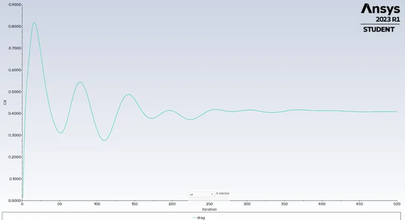
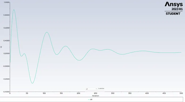
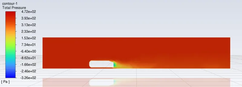
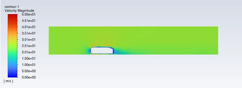
- Simulate the flow with the steady state solver with inlet velocity of 25m/s, with this model having coarse mesh.
Pre-processing:
- From the analysis system toolbox open the Fluid Flow (Fluent)
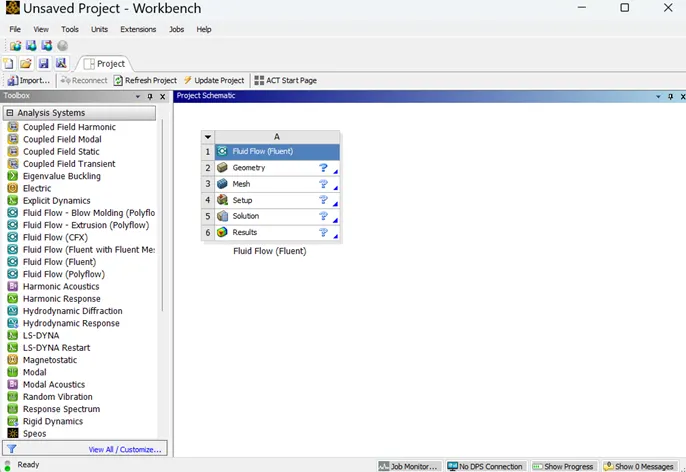
- In Geometry open the spaceclaim for the 2D designing of the model.
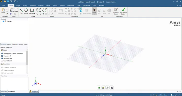
- Geometry of the model is imported.
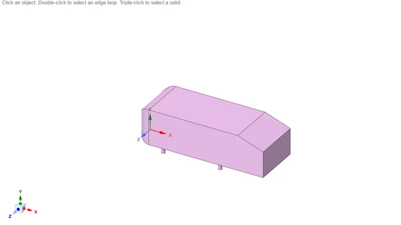
- Create the Enclosure domain for creating flow field around the ahmed body.
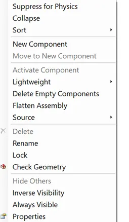
- Suppress the ahmed body for the physics to avoid mesh inside ahmed body.
- Close the spaceclaim and go to mesh. Create the named selection to the model.
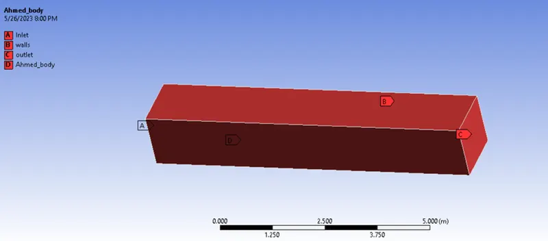
- The default mesh is generated.
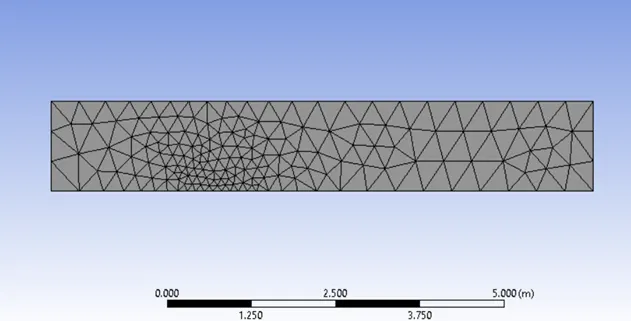
- Solving:
- Open the setup for applying the boundary condition for the fluid flow solution.
|
Setup |
LAMINAR |
|
Solver time |
Steady state |
|
Solver type |
Density Based |
|
Viscous Model |
LAMINAR |
|
Material |
Air o Density- 1.225kg/m3 o Viscosity - 1.7894e-05 Pa s |
|
Boundary Condition |
· Inlet o Velocity- 25m/s · Outlet o Pressure Outlet · Wall o No slip wall. o Stationary wall |
- Scaled residual plots.
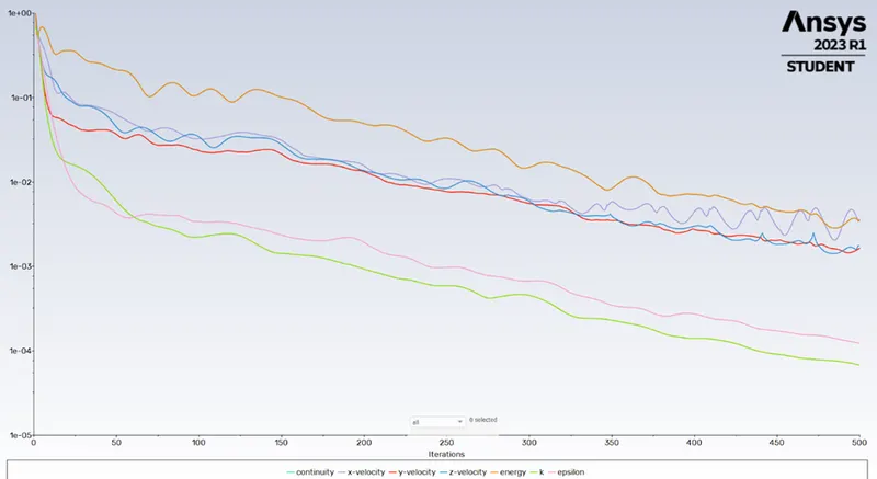
- Co-efficient of Drag plots.
- Co-efficient of lift plots.
- Post-processing:
- Pressure contour:
- Velocity contour:
- Vector plots
CASE 2
- Simulate the flow with the steady state solver with inlet velocity of 25m/s, with this model having refined mesh.
Pre-processing:
- From the analysis system toolbox open the Fluid Flow (Fluent)
- In Geometry open the spaceclaim for the 2D designing of the model.
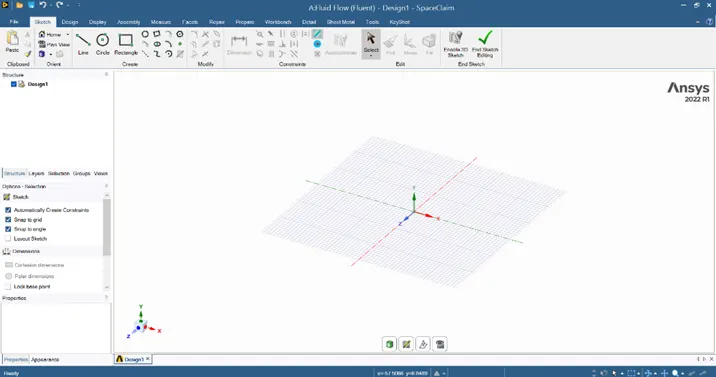
- Geometry of the model is imported.
- Create the Enclosure domain for creating flow field around the ahmed body.
- Suppress the ahmed body for the physics to avoid mesh inside ahmed body.
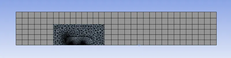
- For the refined mesh create another enclosure near ahmed body.
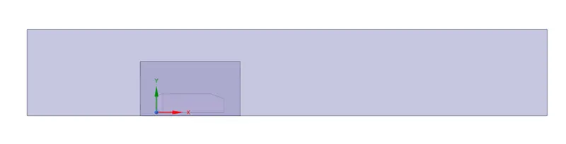
- Rectify interference error between enclosures.
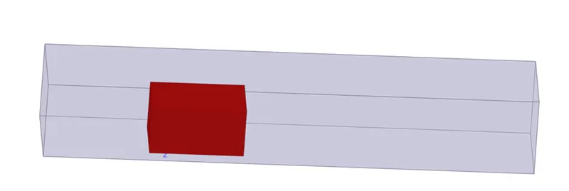
- Close the spaceclaim and go to mesh. Create the named selection to the model.
- The refined mesh is generated.
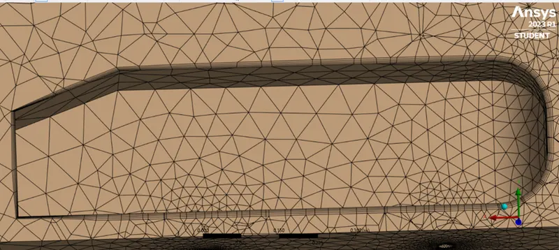
- The inflation up to 5 layers is given around the ahmed body to capture the flow over it.
- Solving:
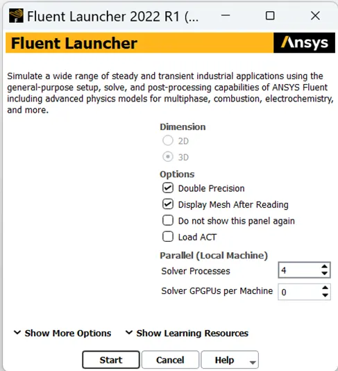
- Open the setup for applying the boundary condition for the fluid flow solution.
|
Setup |
LAMINAR |
|
Solver time |
Steady state |
|
Solver type |
Density Based |
|
Viscous Model |
LAMINAR |
|
Material |
Air o Density- 1.225kg/m3 o Viscosity - 1.7894e-05 Pa s |
|
Boundary Condition |
· Inlet o Velocity- 25m/s · Outlet o Pressure Outlet · Wall o No slip wall. o Stationary wall |
Refined mesh: 1
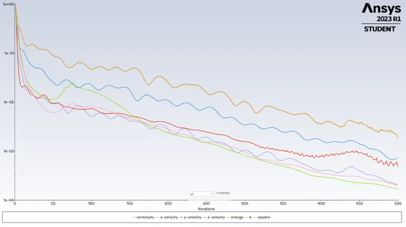
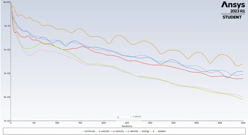
- Residual Plot:
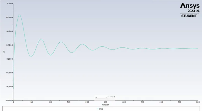
- Coefficient of Drag Plot:
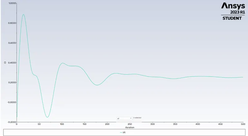
- Coefficient of Lift Plot:
- Post-processing:
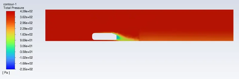
- Pressure Contour:
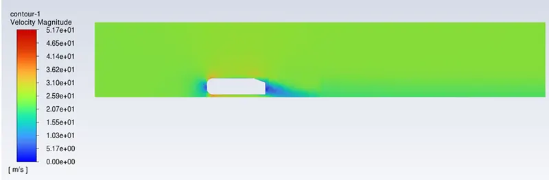
- Velocity contour:
- Vector Plot:
Refined mesh: 2
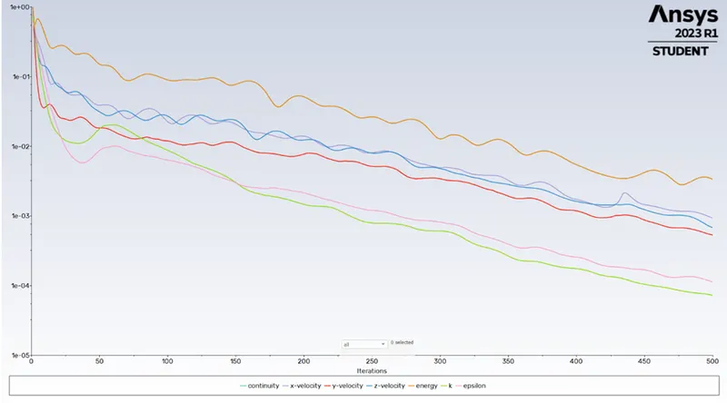
- Residual Plot:
- Coefficient of Drag Plot:
- Coefficient of Lift Plot:
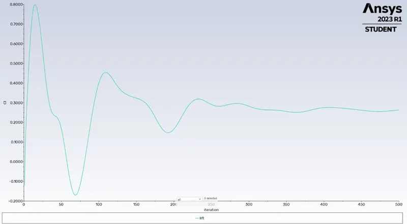
- Post-processing:
- Pressure Contour:
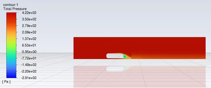
- Velocity Contour:
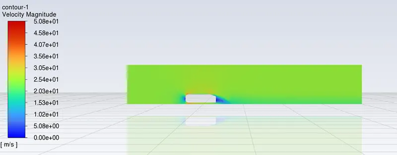
- Vector Plot:
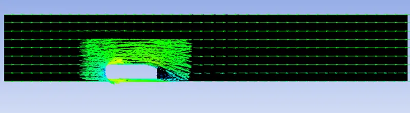
Refined mesh: 3
- Residual Plot:
- Coefficient of Drag Plot:
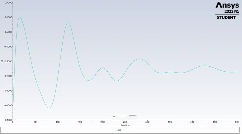
- Coefficient of Lift Plot:
- Post-processing:
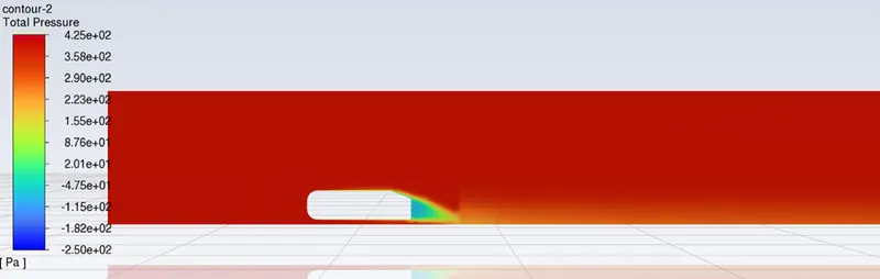
- Pressure Contour:
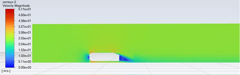
- Velocity Contour:
- Vector Plot:
Comparison table:
|
Refined mesh |
Mesh sizing |
Elements |
Cl |
Cd |
|
|
Inner (m) |
Outer (m) |
||||
|
1 |
0.100 |
0.250 |
90750 |
0.2531 |
0.3481 |
|
2 |
0.75 |
0.200 |
103754 |
0.2627 |
0.3395 |
|
3 |
0.50 |
0.150 |
167759 |
0.2283 |
0.3086 |
Conclusion:
- From the grid independence study results, I conclude that refining mesh size finer increasing the accuracy of the stimulation results.
- It results that lift increases and drag decreases accordingly.
- The negative pressure created at the wake region of the ahmed body due to less shear stress near the boundary layer.
Reference Paper
- https://www.researchgate.net/publication/266883948_Flow_and_Turbulence_Structures_in_the_Wake_of_a_Simplified_Car_Model_Ahmed_Model
- https://www.researchgate.net/publication/330383775_Experiments_and_numerical_simulations_on_the_aerodynamics_of_the_Ahmed_body
- https://www.comsol.com/blogs/studying-the-airflow-over-a-car-using-an-ahmed-body/
- http://wwwmdp.eng.cam.ac.uk/web/library/enginfo/aerothermal_dvd_only/aero/fprops/introvisc/node9.html