Week 3 - External flow simulation over an Ahmed body.

AIM :-

• External Flow Simulation Over an Ahmed Body Using Ansys Fluent.

OBEJECTIVE :- 

•  Need to use the 'Split Body' command in SpaceClaim to perform the operation and symmetry boundary condition in fluent to perform the simulation. 
•  To Run the Simulation for the Velocity of 25 m/sec with the default air properties in fluent.
•  Describe Ahmed's body and its Importance.
•  Explain the Reason for the Negative Pressure in the Wake Region.
•  Explain the Significance of Point Of Separation.

EXPECTED RESULT.

•  Velocity and Pressure Contour.
•  The Drag Co-efficient plot of refined Case. ( For Velocity 25m/s the Drag Coefficient should be around `C_d`0.33)
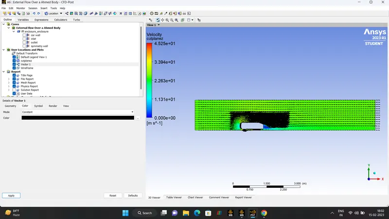
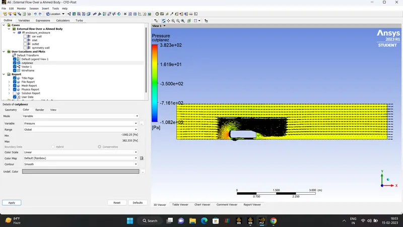
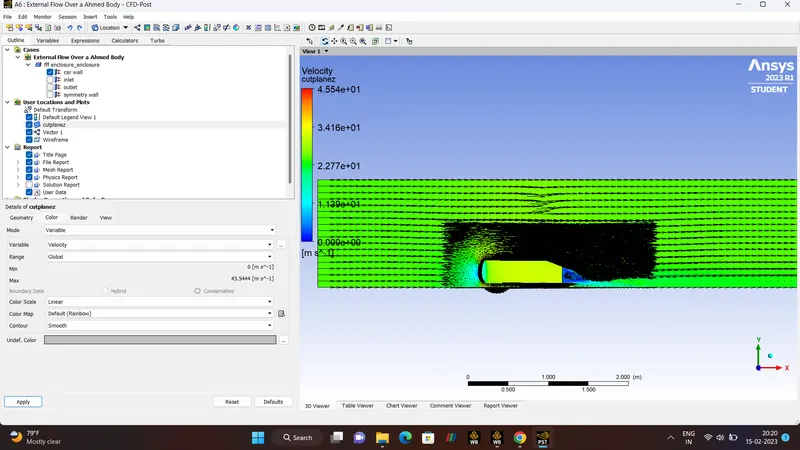
•  The Vector Plot clearly showing the Wake Region.
•  Grid Independence test and provide the value of Drag and Lift Co-efficient.

                                        AHMED BODY.

                                        DRAG / LIFT CO-EFFICIENT.

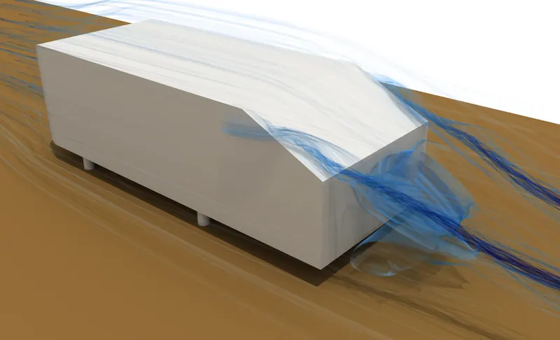
                                        WAKE.

                                        POINT OF SEPERATION.

• AHMED BODY.  

                                                      

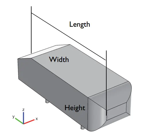
INTRODUCTION:-

• Ahmed body was first created by S.R AHEMD in his Research 'Some Salient Feature of Time-Averaged Ground Vehicle Wake' in the year of 1984.
• Since then it has become a benchmark for widely used in Automobile Industry for Validating the Aerodynamic tools.
• The Ahmed body Shape is simple enough to model, while maintaining Car-Like Geometry feature.
• The particular goal of this benchmark is to Calculate the Drag-Coefficient, Velocity Profiles, Velocity field and Time Averged Wake Structure. 
• The body signifies a simple type, ground Vehicle geometry of a bluff body type with slant back and rear back.
• Ahmed body is made up of round part of movable slant plane placed in rear end of body to learning the partition phenomena at different angle and the rear slant plane and wake flow a ahead of the ahmed body. 
• It has industrialized into a standard point of reference Reynold's Average Navier-Stroke Equation model.
• As the Wake flow behind the Ahmed Body is the main contributor to the force, accurate prediction of the separation process.
• To Simulate the Wake Flow accurately, resolving the near wall region using accurate turbulence model is highly desirable.
• Both the K-OMEGA and K-EPISLON model can be used, but in our case going to use the K-EPISLON model.  

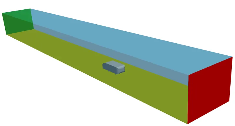
WIND TUNNEL REPRESENTATION.

                                    

• DRAG CO-EFFICIENT.

DEFINITION:-

• Drag Co-efficient is a dimensionless quantity used to measure the Drag or Resistance of an Object in Fluid Environment such as Water or Air.
• The forumla for Drag Co-efficient is expressed as  

                                                                  `C_d = F_d /(0.5*rho*a*v^2)`

`C_d : Drag Coefficent .`

`rho : Density.`

`F_d : DRAG FORCE`

`a : Area.`

`v^2 : Flow Velocity.`  

WHY DO WENEED DRAG COEFFICIENT IN CARS.

• It is not an absolute constant for a body's shape because it varies with Speed and Direction of flow, Object Shape, Size and Density, Viscosity of Fluid.
• The lower the Drag Co-efficient of an Object, the less Aerodynamic or Hydrodynamic Drag Occurs.
• In term of Car, the lower the Drag Co-efficient the more efficient car is. As well as affecting the top-speed of a vehicle, the Drag Co-efficient also affects the handling.
• Car's with lower drag co-effcient are sought after, but decreasing the drag drasticallycan reduce the downfall and leads to loss in road traction and higher chance of car accidents.
• Most Car's have an Average Drag Co-efficient of between 0.30 and 0.35.
• Boxy Cars have Higher number like HUMMER H2 Vehicle at 0.57.
• Streamlined and Agile Car have Lower Number like MERCEDES-BENZ C-CLASS Vehicle at 0.24.
• This is average, the exact Drag Co-efficient Varies with REYNOLD's NUMBER and Varies Other Factor. 

FOR EXAMPLE :-

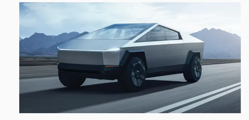
• TESLA CYBERTRUNK has a DRAG Co-efficient of 0.39

                                                

• LIFT CO-EFFICIENT.

DEFINITION:-

• Lift Co-efficient is a dimensionless quantity used to measure the lift of an Object in Fluid Environment.
• The forumla for Lift Co-efficient is expressed as                                                    

                                                                  `C_l = F_l /(0.5*rho*a*v^2)`

`C_l : LIFT CO EFFICIENT .`

`rho : Density.`

`F_l : LIFT FORCE`

`a : Area.`

`v^2 : Flow Velocity.`

• WAKE. 

                                             

DEFINITION:- 

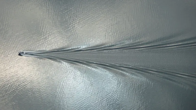
• Wake is defined as region of recirculating the flow immediately behind a Moving or Stationary Blunt Body caused by Viscosity which may be accompained by flow Seperatoin and turbulence (or) the Wave Pattern on a Water DownStream of an Object in a flow, or Produced by a moving Object (eg Ship) caused by Density Difference of the Fluid above and below free Surface and Gravity or Surface tension.

                                             

• FLOW SEPARATION.

DEFINITION:-

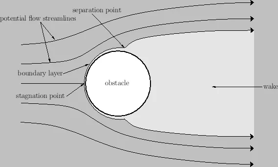
• Flow Separation or Boundary Layer Separation is the detachment of a boundary layer from a surface into a wake. A boundary exists whenever there is relative movement between the fluid and solid surface with the viscous forces present in the layer of the fluid close to the surface. A boundary layer can either Laminar or turbulent flow, It is calculated based on the Reynold's number.

POINT OF SEPARATION.

• Separation occurs in the flow that is slowing down with pressure increasing, after passing the thickest part of the streamline body. Flowing against an increasing pressure is known as flowing air in an adverse pressure gradient. The boundary layer separates when it has travelled far enough in an adverse pressure gradient that the speed of the boundary layer relative to the surface has stopped and reversed direction. The Flow becomes detached from the surface and instead forms a eddies or vortices. In aerodynamics the flow separation results in reduced lift and increase pressure drag, caused by the pressure differential between the fornt and rear end surfaces of the body.

• DENSITY-BASED SOLVERS.

DEFINITION:- 

• Density Based Solvers was developed for High-Speed Compressible flows.
• It solves the Energy, Momentum,Continuity and Species Transport equation Simultaneously.
• This solvers is best suitable for Supersonic Flow.
• This Solvers is used when 'MACH NUMBER' is greater than 0.3. 

• PRESSURE-BASED SOLVERS.

DEFINITION:- 

• Pressure Based Solvers was developed for Low-Speed Incompressible Flows (M<0.3) and mildly Compressible Flow.
• This solver uses Momentum and Pressure as the Primary variables. 

There are two types,

• Pressure Based Segregated Algorthim.
• Pressure Based Coupled Algorthim.

In Algorthim there are Five Types,

COUPLED.

SIMPLE.

SIMPLEC

PISO

FMS.

In our case we are going to use the Pressure Based Solver where the Energy is Turned off.

• GEOMETRY.

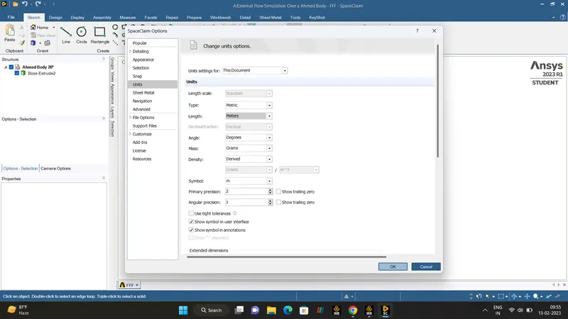
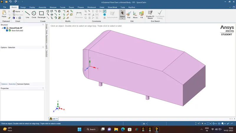
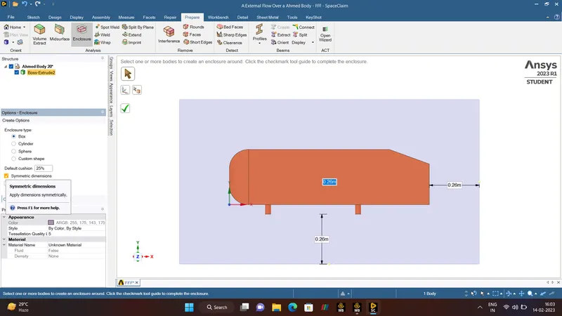
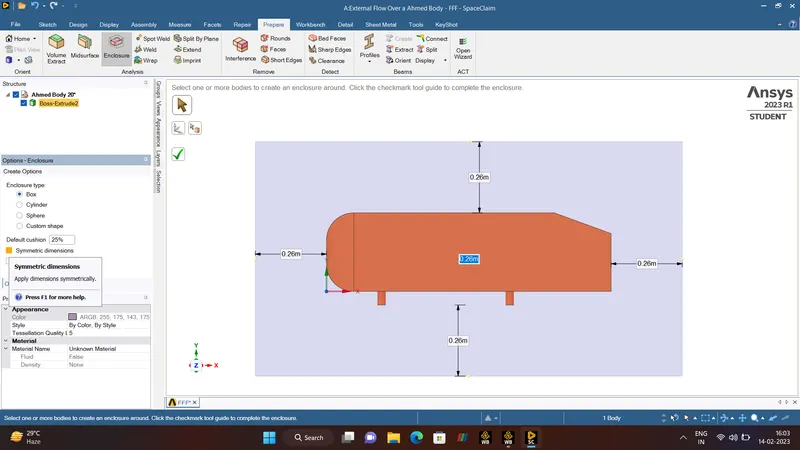
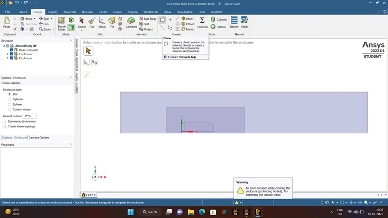
In Geometry Section First we need to import the AHMED BODY, then need to create the ENCLOSURE with respect to the Dimensions. So far Enclosure just go to the PREPARE Tool and click the ENCOSURE Option then the Ahmed Body. Change the UNITS  from Millimeters into Meters.

      

• FIRST ENCLOSURE.

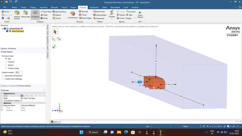
In First Enclosure, UnClick the Symmetric Dimensions and give the dimensions respectively.

Width for Both Sides are 0.5m, towards the y direction 1m, and for x directions 2m and 5m.

     

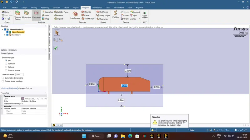
• SECOND ENCLOSURE.

1m and 0.5m for x direction and 0.5m for the y direction.

  

• PLANE.

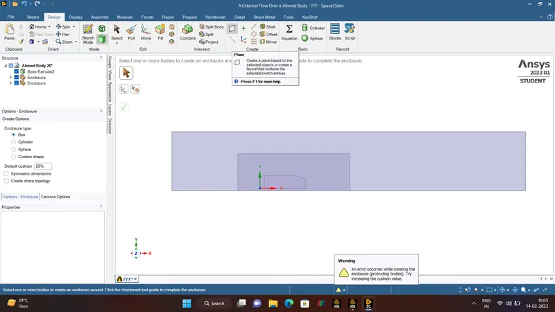
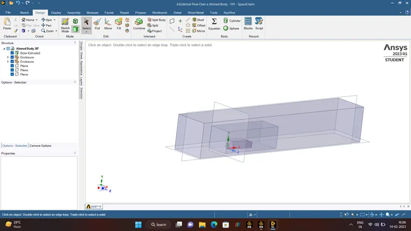
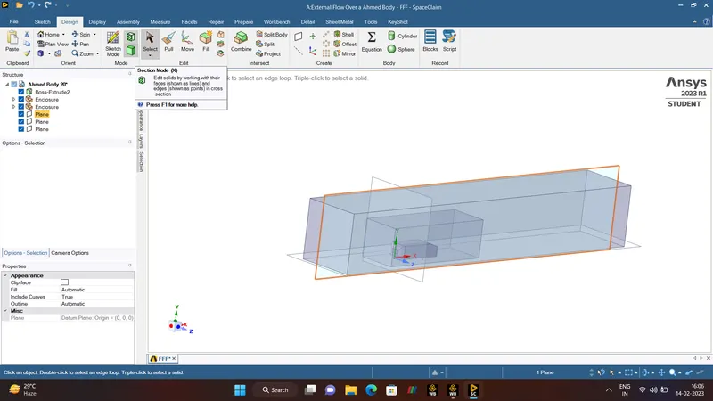
The Plane tool is selected for the hatching process to check the interference

     

• HATCHING.

Before.

    

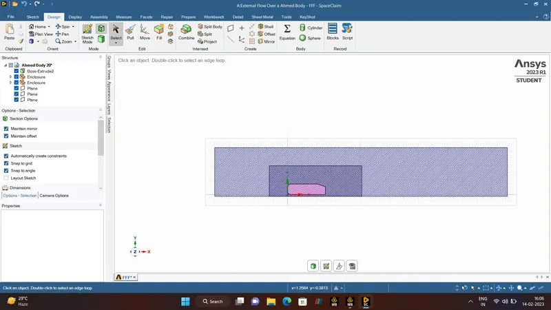
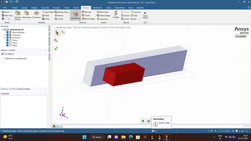
After.

     

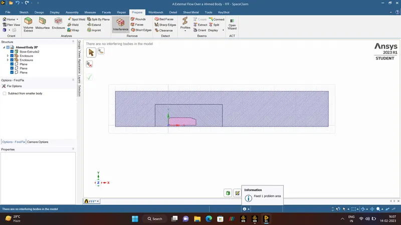
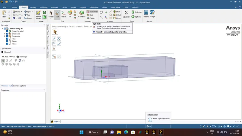
• SPLIT BODY COMMAND.

Split body command is used for splitting the bodies into the half as it is symmetry shape. so it takes much less time for the computational time.

    

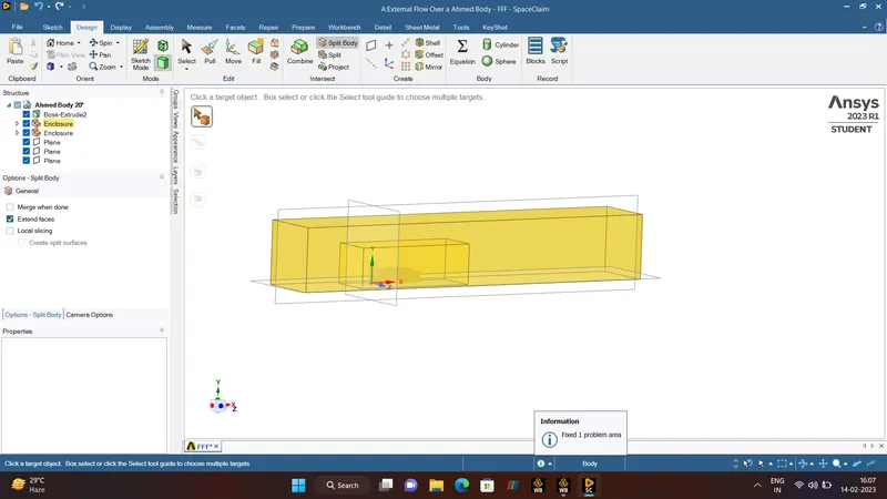
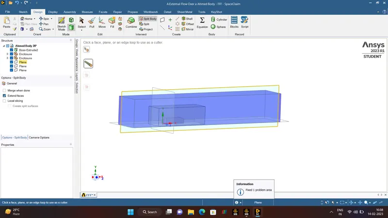
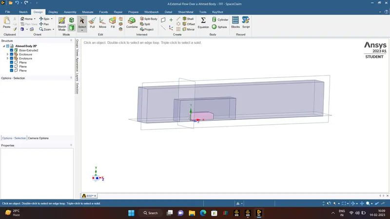
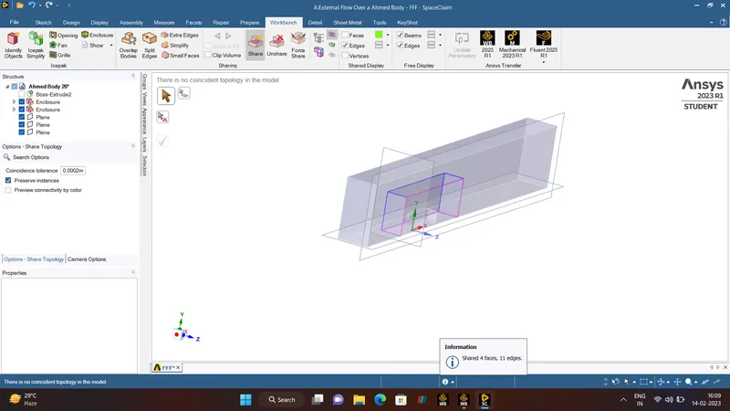
In Same do for the remaining bodies. and finally Share topology is used before doing the share topology need to click the ahmed body which we made into supress for physics.

 

• MESHING.

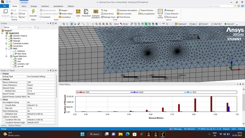
Meshing is the major part of Engineering simulation process. Here are the larger geometry is discretized into the small simple elements in Order to get the accurate solution.

 

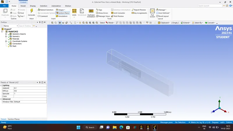
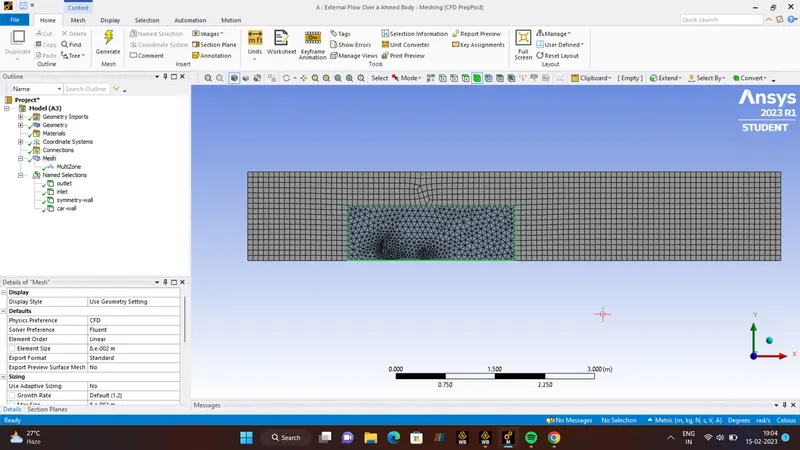
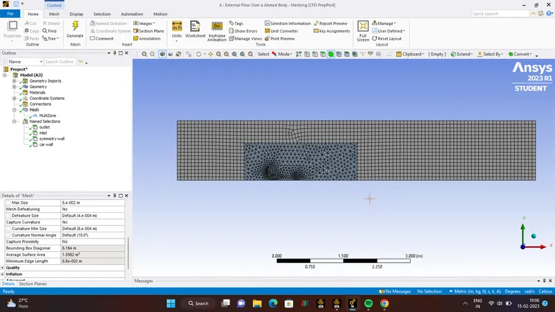
First Generating the normal mesh and Check, In the First Image it is clearly Shown that the Meshing is Overlapping and Unstructured that's because we did'nt do the  Hatching process 

    

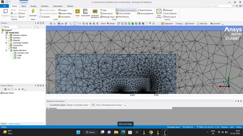
After Hatching Process is done we can clearly able to see the Mesh is Uniform.

 

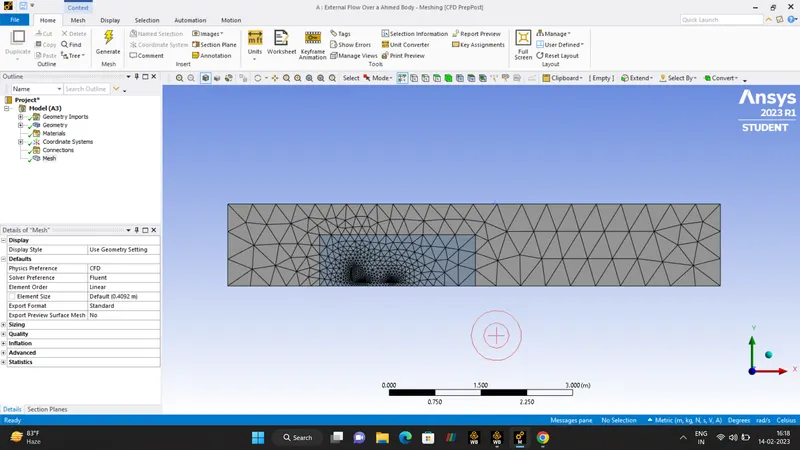
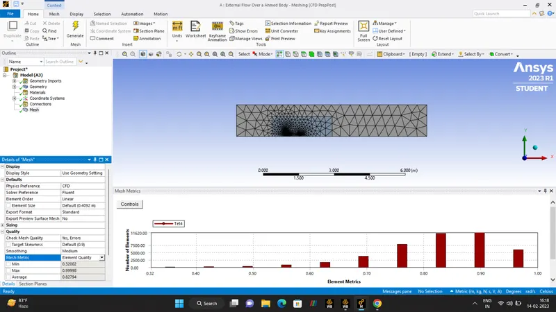
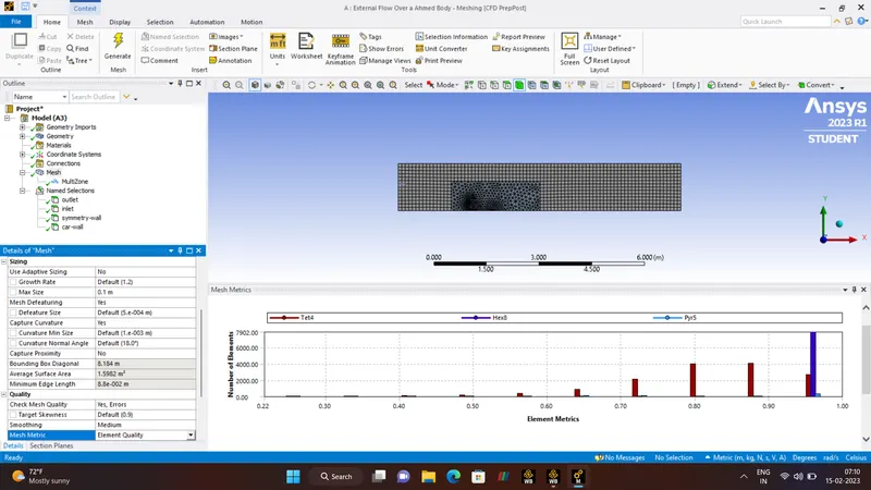
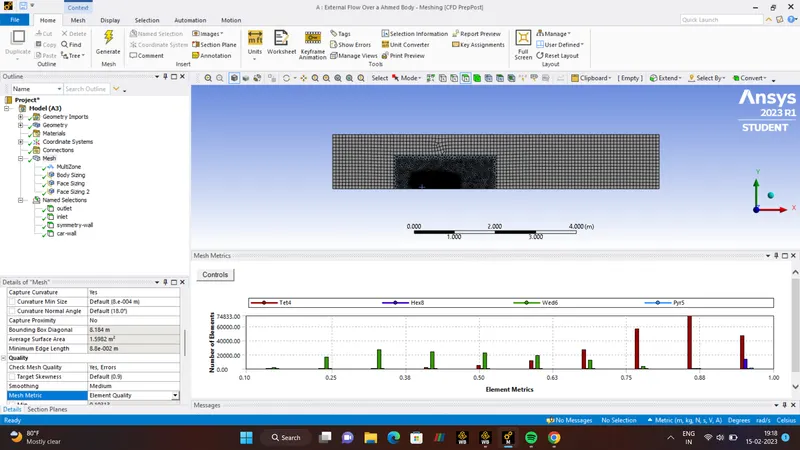
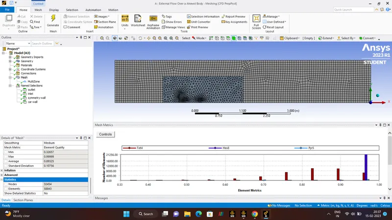
• MESH QUALITY.

 

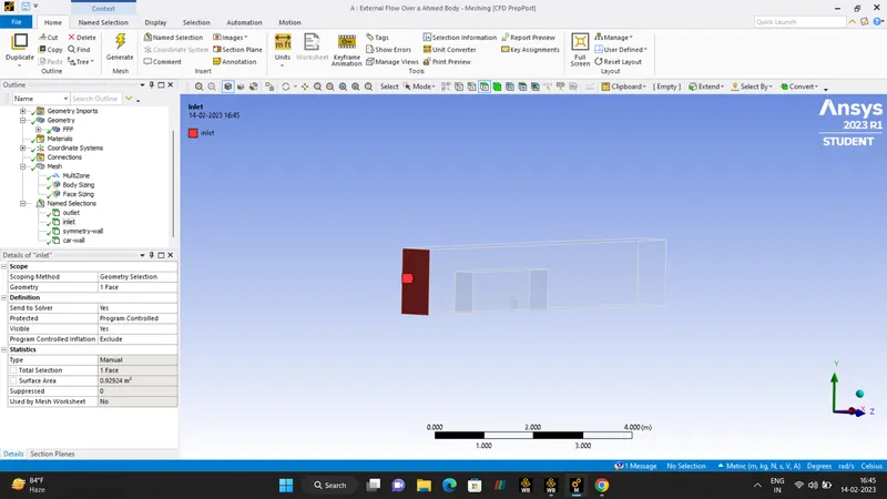
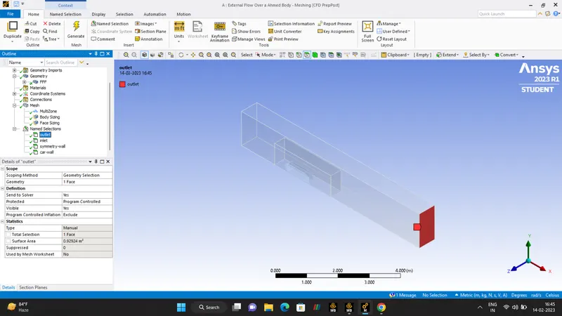
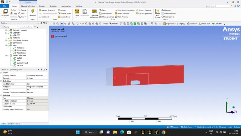
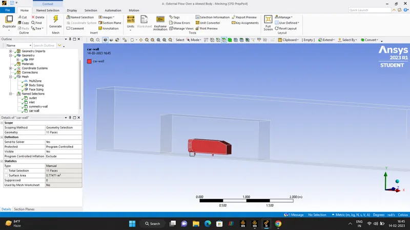
• NAME SELECTION.

                                     1.  INLET.

                                     2. OUTLET.

                                     3. SYMMETRY WALL.

                                     4. CAR WALL.

For Name Selection Process click the face selection tool (Ctrl+F) and give the names respectively. And for the car-wall need to the hide the faces of both the Enclosures and with the help of the BOX SELECT tool name is been given.

                                                                   

        

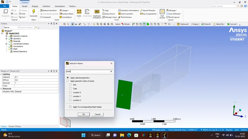
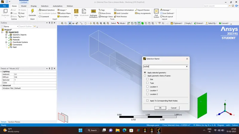
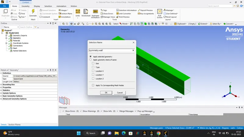
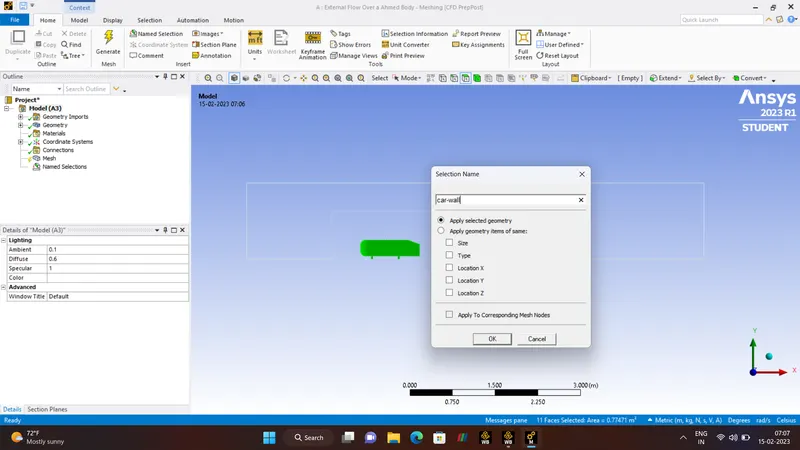
Before proceeding with the next Step click the Name Selection again. 

    

• METHOD.

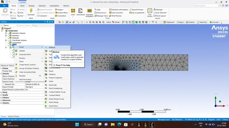
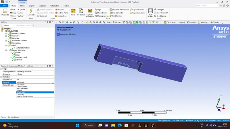
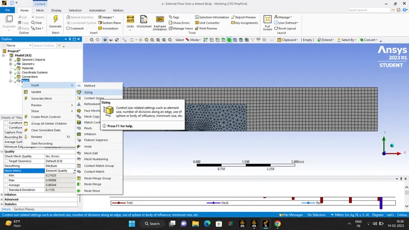
Right Click on the MESH and select INSERT, after selecting the INSERT click on the METHODS, After Clicking the methods will find the dialog box at the left side of the bottom, In that dia box the SCOPE and DEFINITION, In that Scope option have to select the geometry in order to do the mesh.

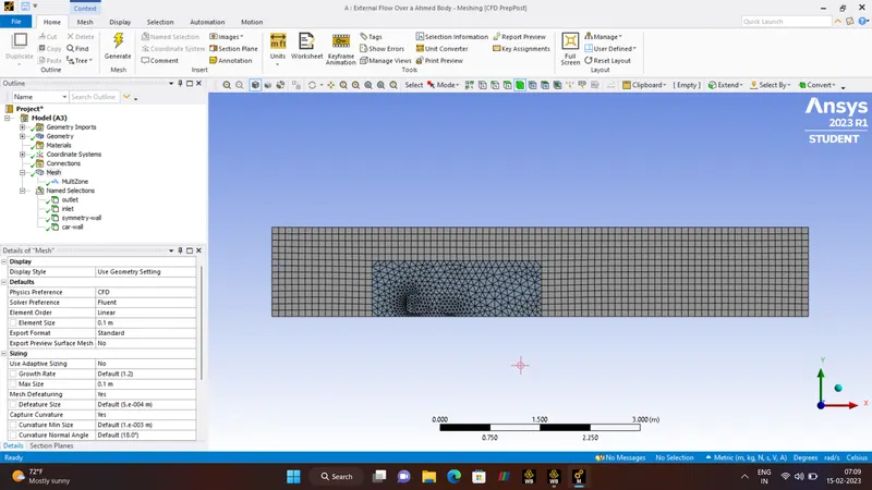
There are 6 methods available in the methods in our case we are going to use the MULTIZONE Method. HEXAHEDRON mesh highest quality mesh.

Element Size - 100mm = 0.1m

Max Element Size - 100mm = 0.1m

  

 

  

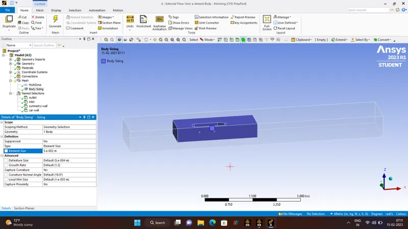
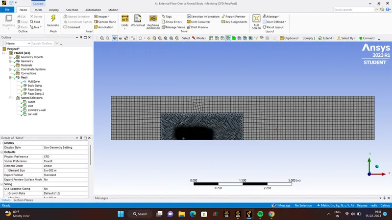
• SIZING.

same as method Sizing is done.

Element Size 50mm = 0.05m.

 

Face Sizing element Size 10mm = 0.01m

      

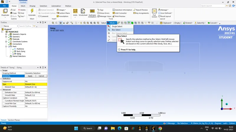
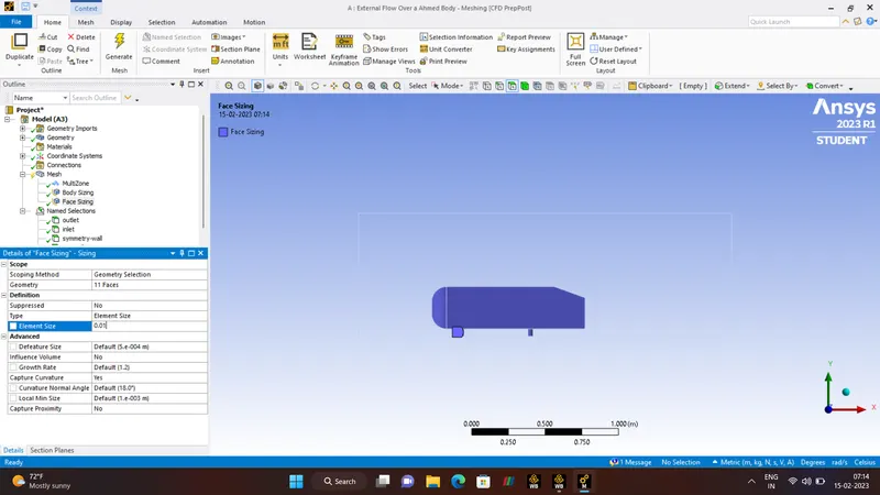
 4 Face legs has been Selected and the Element Size is 5mm = 0.005m

 

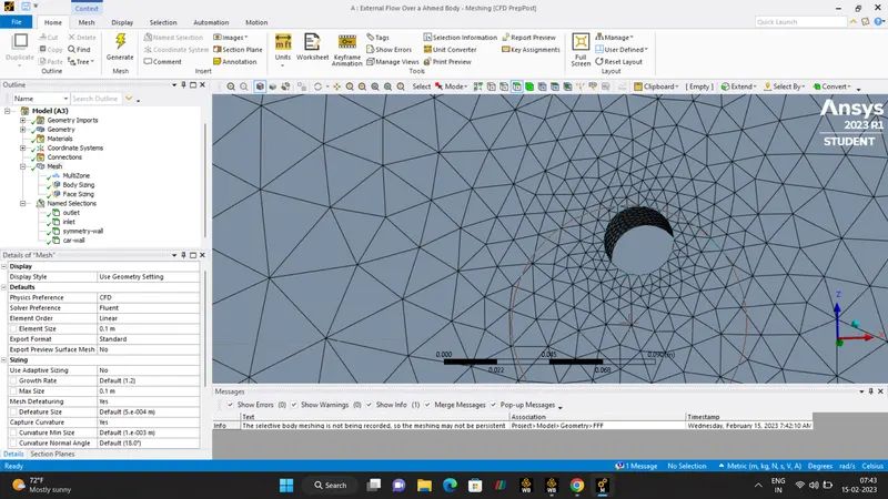
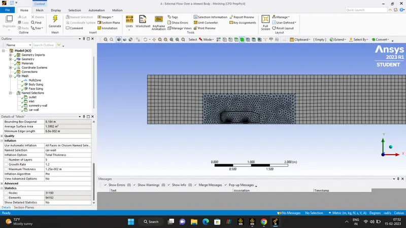
• INFLATION.

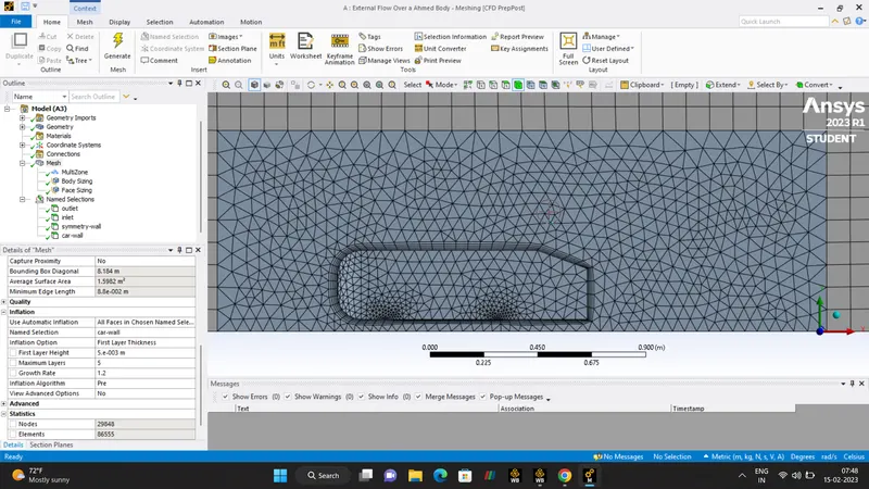
Inflation layers are given because the real Gemoetry are complex and often to use an Unstructured mesh. Unstructured Meshes are not thin close to the wall.

Inflation layers are the fine layers of mesh around the domain.

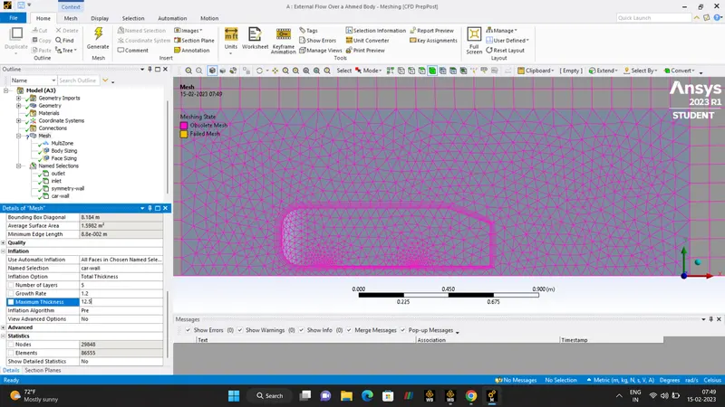
Inflation layer 5.

Total thickness is 12.5mm

 

 

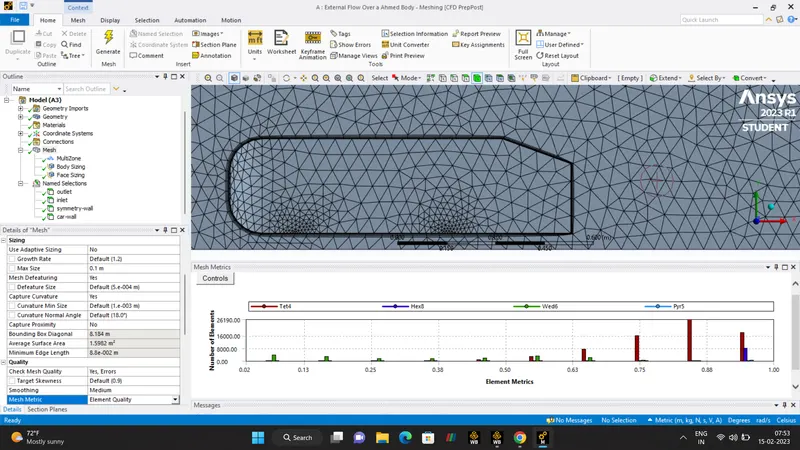
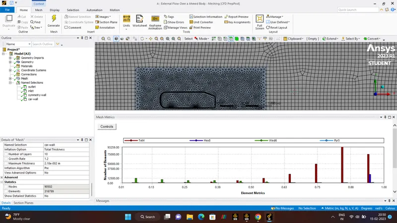
• NUMBER OF NODES AND ELEMENTS.

Number of Nodes - 31190

Number of Elements - 94192

 

• SETUP.

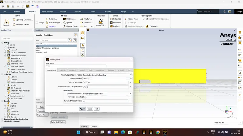
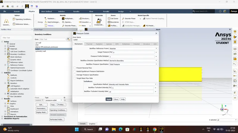
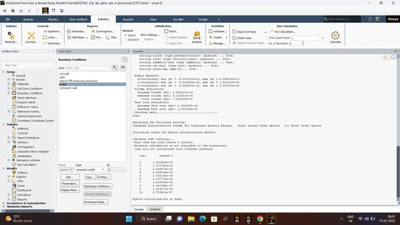
In our case we going to select the PRESSURE BASED SOLVER.

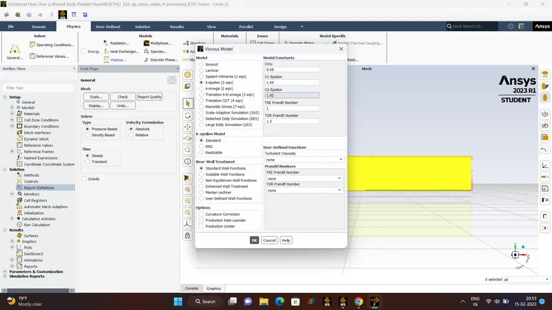
K-EPSILON model.

INLET VELOCITY - 25m/s.

MATERIAL - AIR.

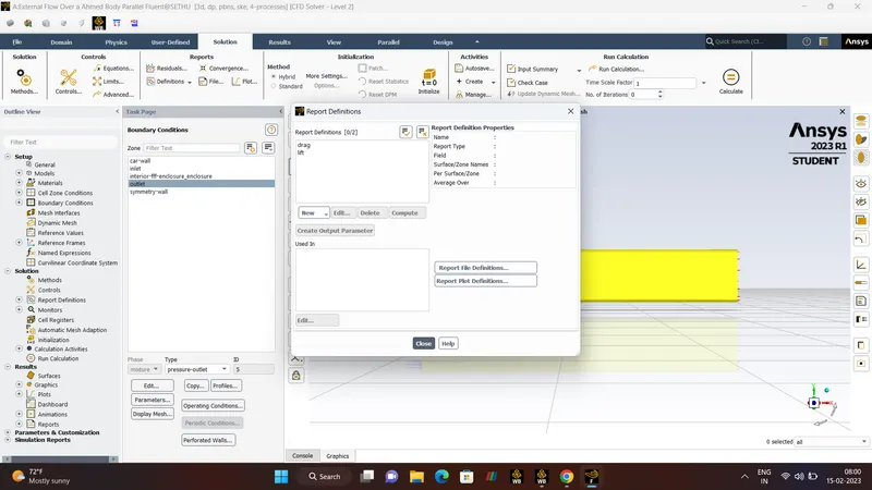
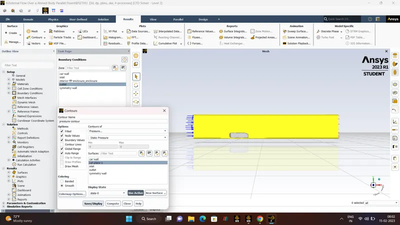
REPORTS - Drag, Lift, velocity and Pressure Contours.

 

     

    

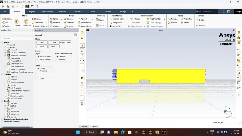
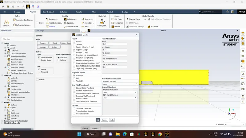
• RESULTS.

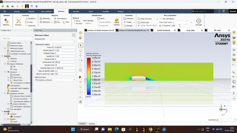
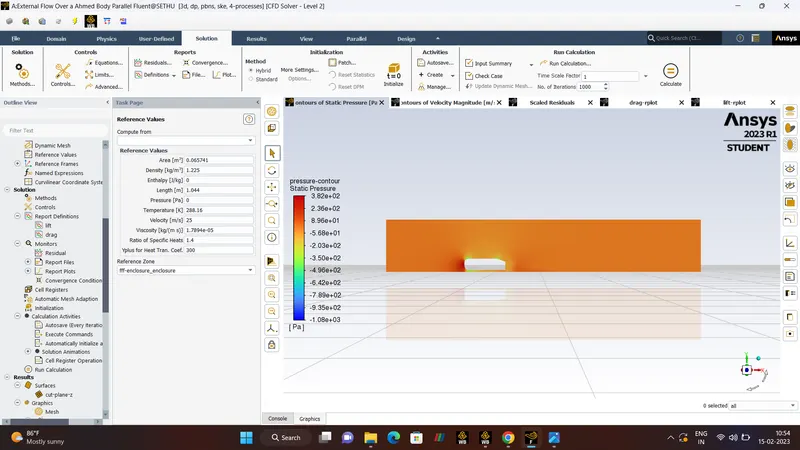
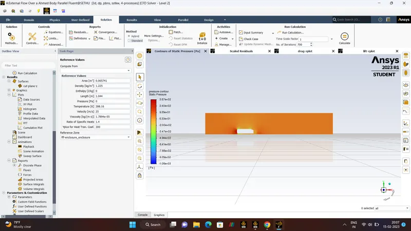
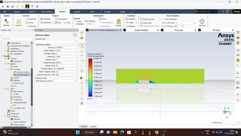
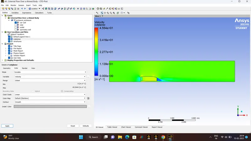
Velocity and Pressure Contour.

 

Residuals.

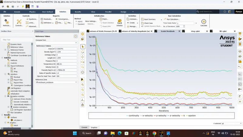
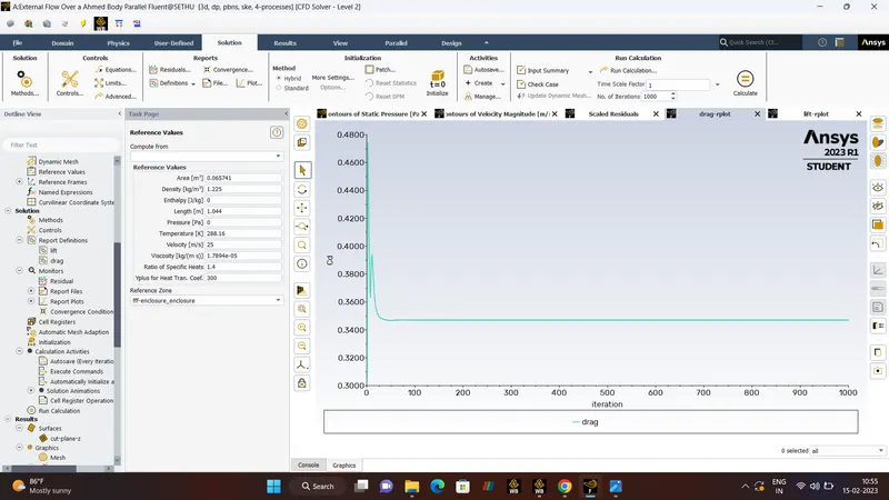
Drag Co-efficient.

 

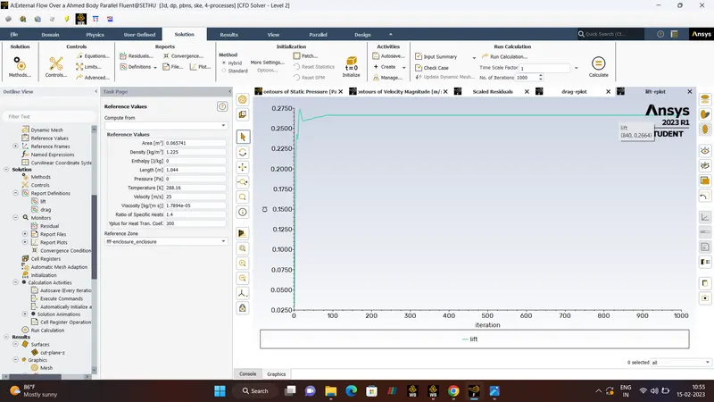
Lift Co-efficient.

 

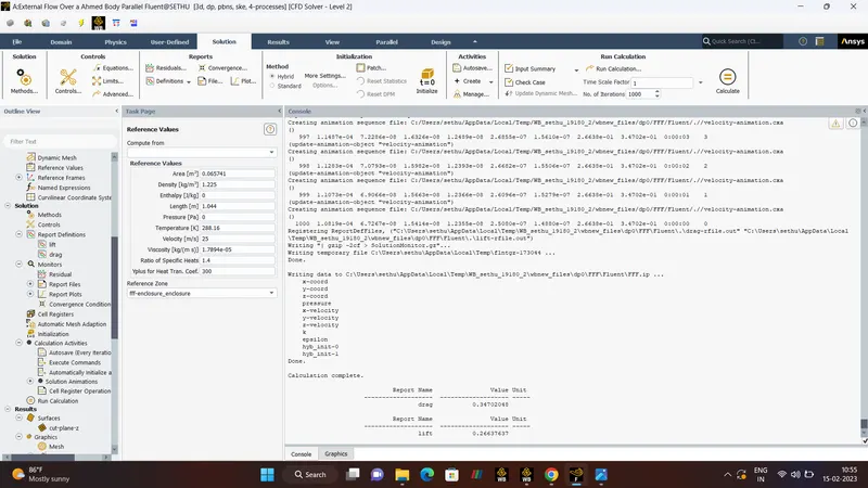
Drag and Lift .

Drag Co-efficient - 0.34

Lift Co-efficient - 0.26

• POST-PROCESSING.

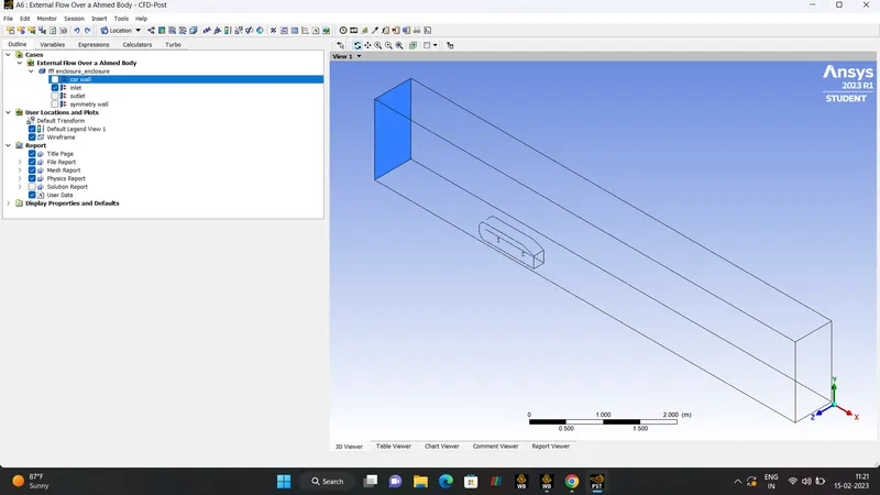
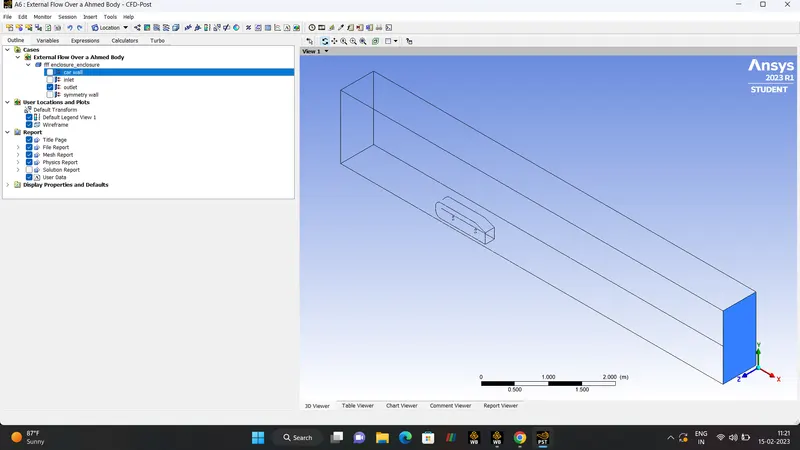
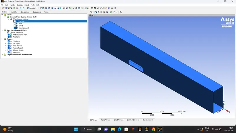
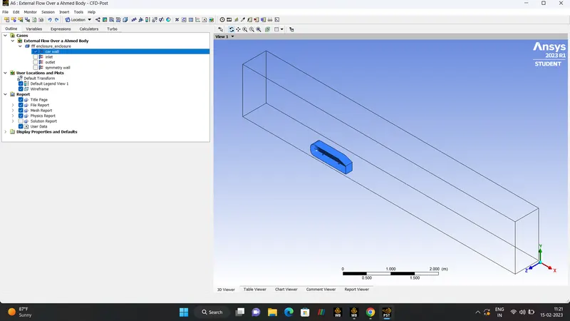
 Inlet, Outlet, Car-Wall, Symmetry-Wall.

      

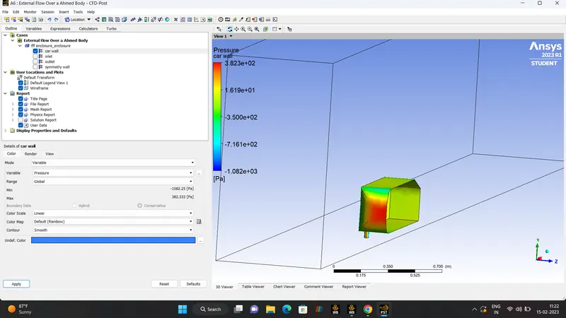
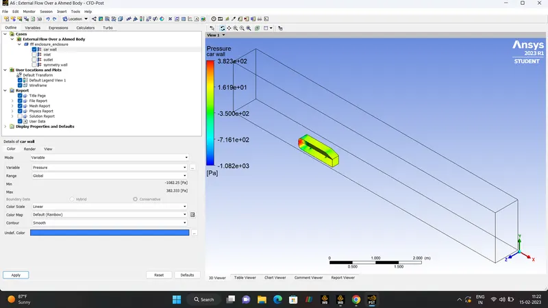
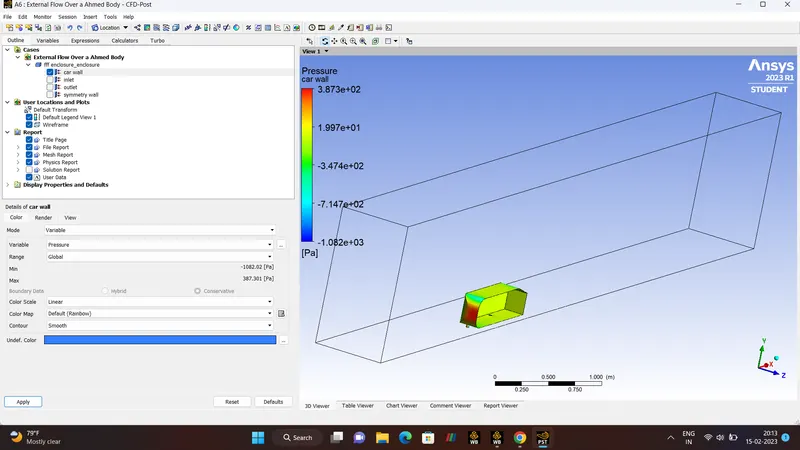
Pressure Car-Wall.

 

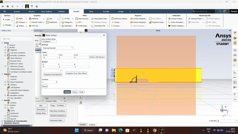
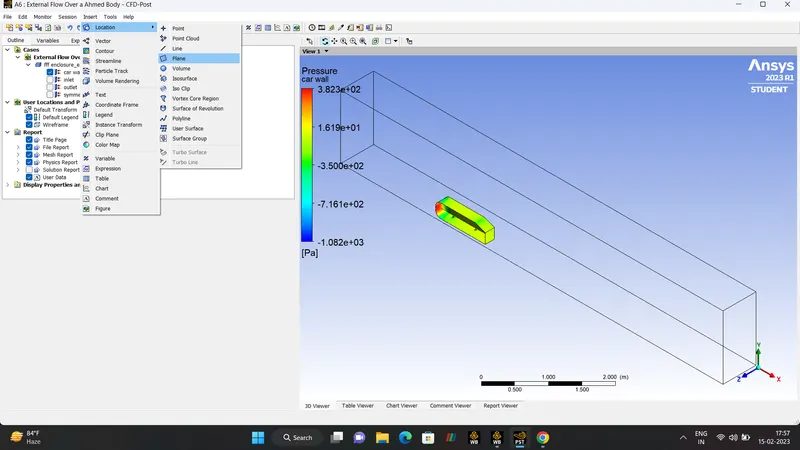
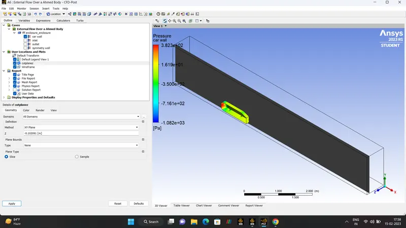
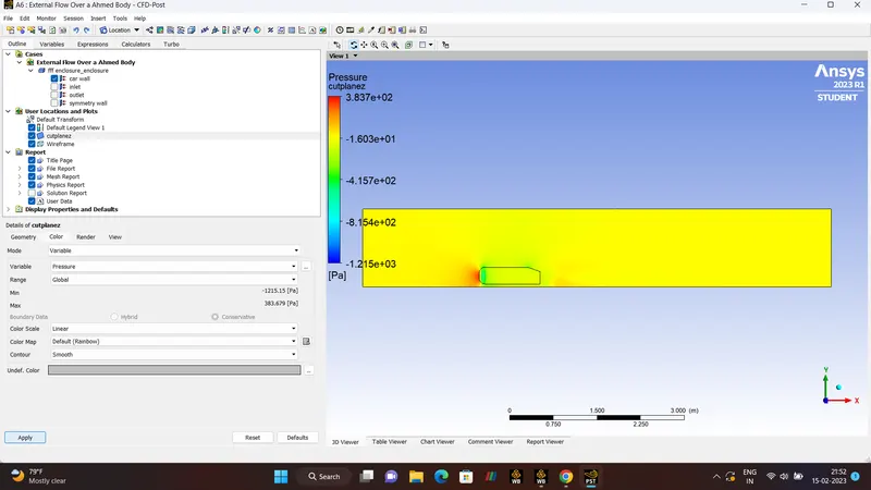
 CutPlaneZ (YX Axis).

  

Velocity

 

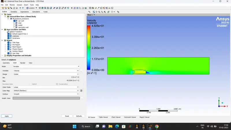
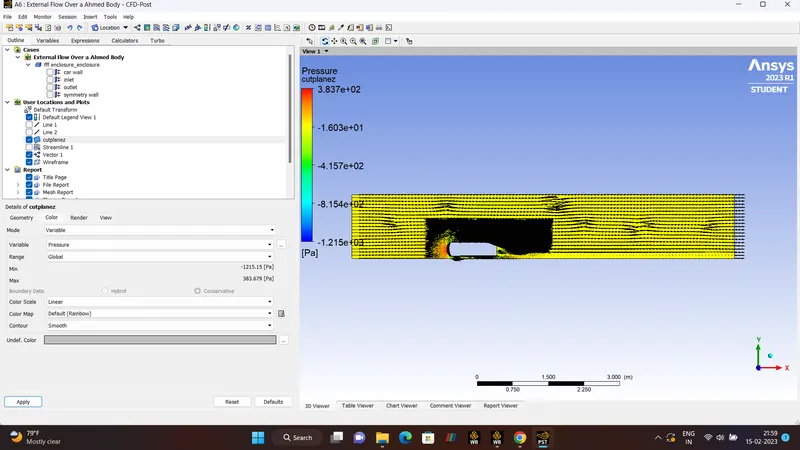
Velocity Vector. 

 

 

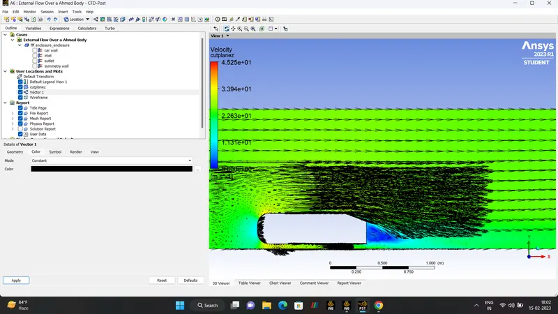
Pressure.

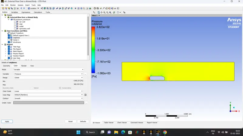
Pressure Vector.

 

CASE-2 :-  GRID INDEPENDENCE 

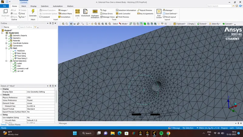
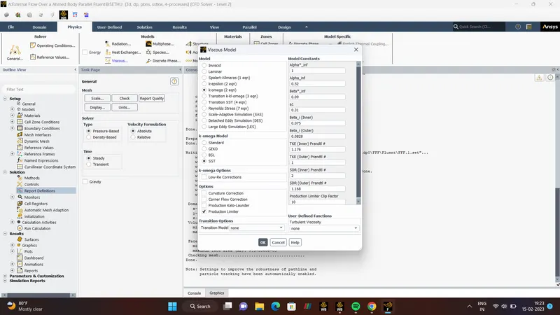
• K-OMEGA MODEL. (TURBULENCE FLOW)

METHOD - Multizone 

Element Size - 80mm =0.8m.

Max Element Size -80mm = 0.8m.

BODY SIZING- Element Size - 40 mm =0.04m

FACE SIZING - Element Size - 5mm = 0.005m

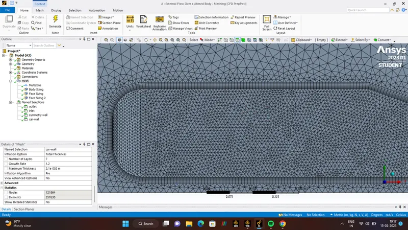
INFLATION 

First Cell Height - 0.00014m

Total Thickness-0.0218m

Number Of Layers - 7

RESULTS.

Number Of Iteration - 700.

Drag - 0.29

Lift - 0.21

 

  

 

 

 

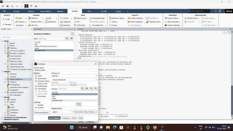
Results. 

 

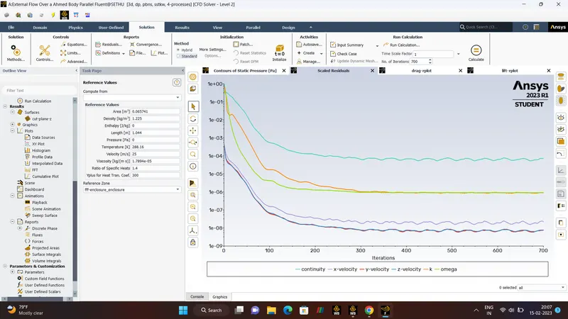
Drag Co-efficient.

 

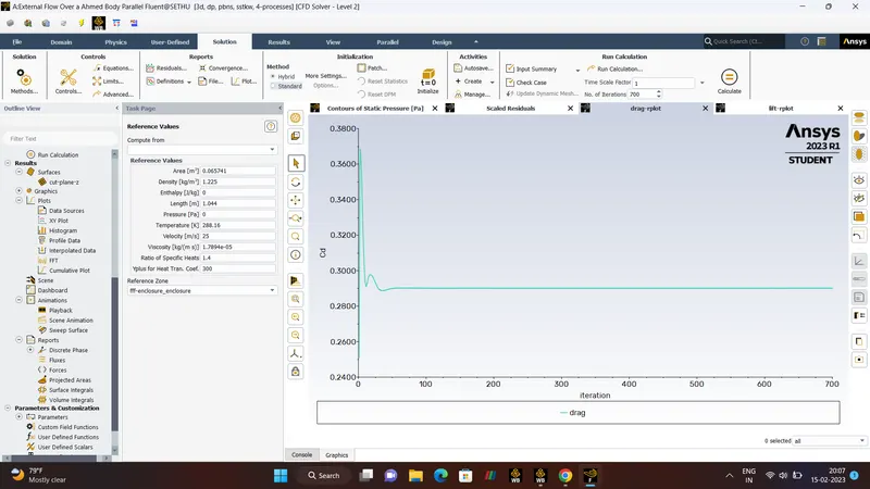
Lift Co-efficient.

 

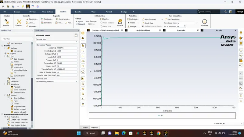
DRAG and LIFT RESULTS.

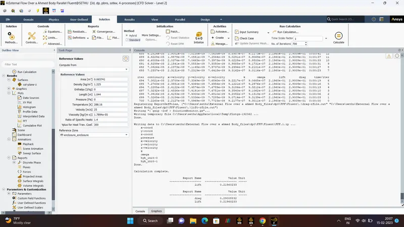
Pressure Contour.

 

Velocity Contour.

 

CFD-POST.

 

Velocity and Vector Plane.

  

Pressure and Vector.

 

 

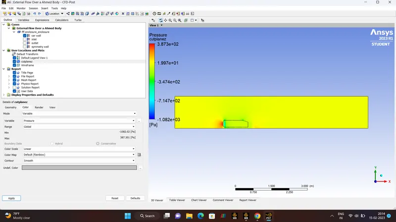
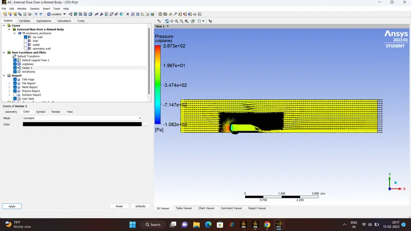
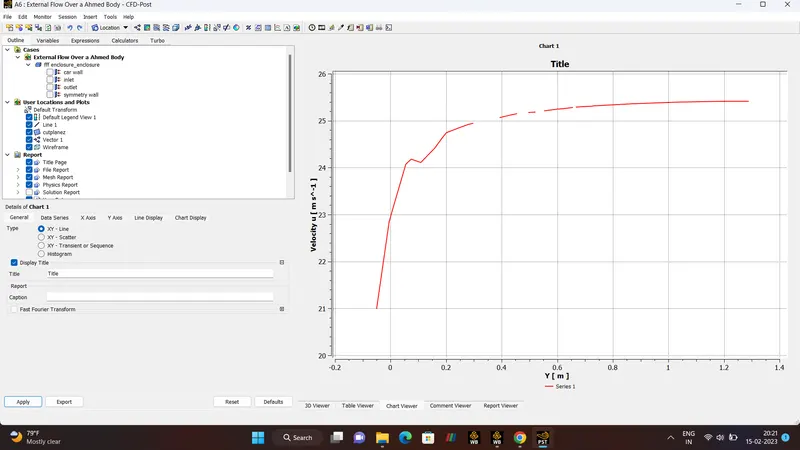
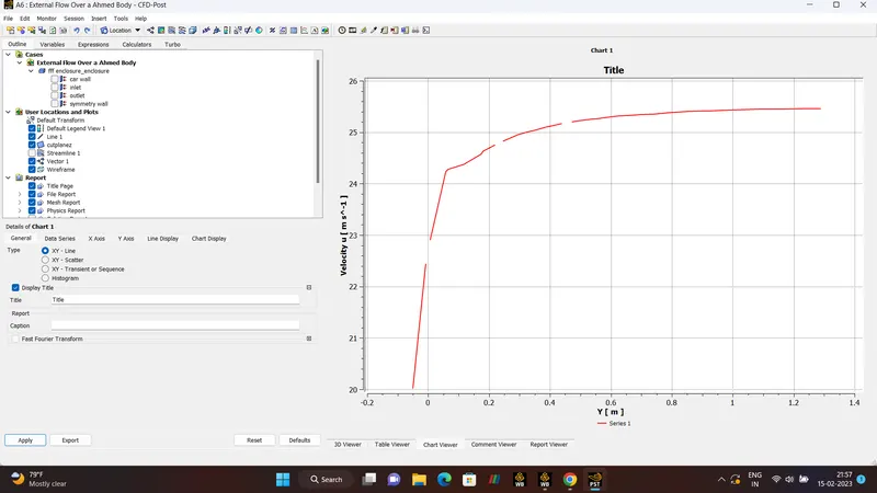
 Chart. (VELOCITY u) 

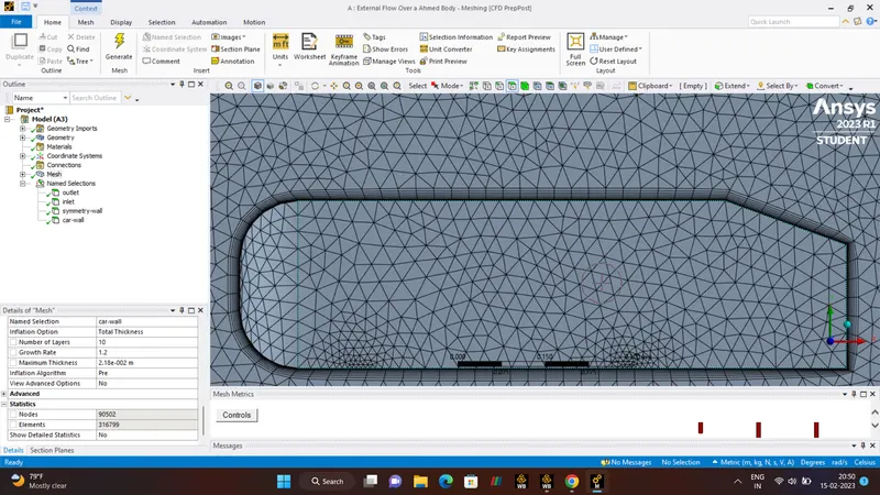
CASE-3 :-

 TURBULENCE = K-EPSILON MODEL.

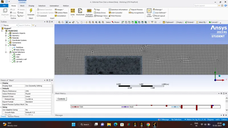
METHOD - Multizone 

Element Size - 70mm =0.7m.

Max Element Size -70mm = 0.7m.

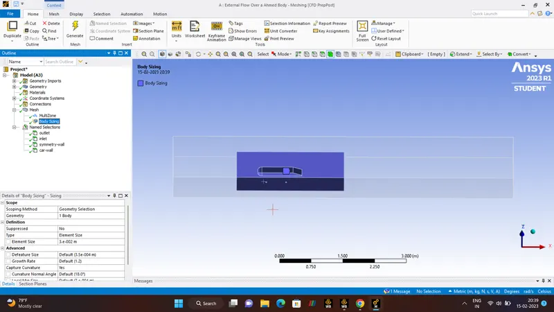
BODY SIZING- Element Size - 30 mm =0.03m

FACE SIZING - Element Size - 5mm = 0.005m

INFLATION 

First Cell Height - 0.029m

Total Thickness-0.021m

Number Of Layers - 10

Y+ = 200.

RESULTS.

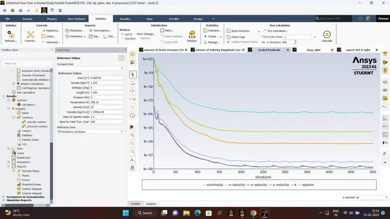
Number Of Iteration - 500.

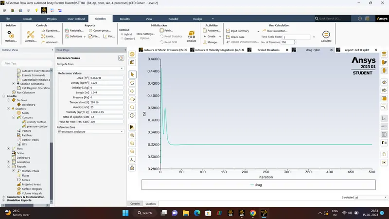
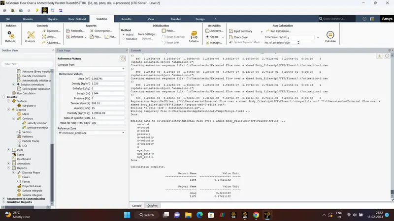
Drag - 0.32

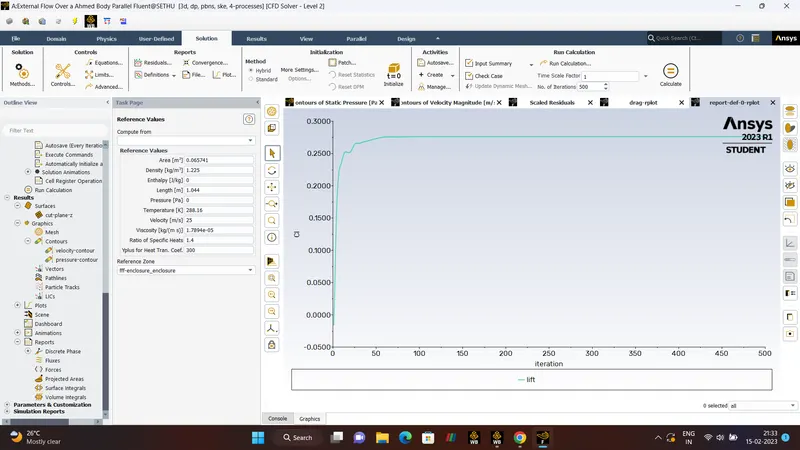
Lift - 0.27 

 

 

 

 

 

 

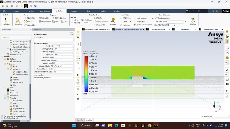
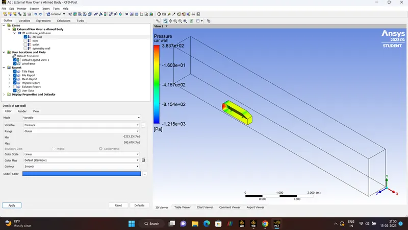
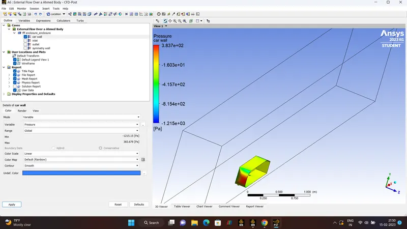
Pressure Contour. 

 

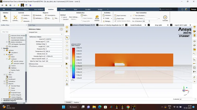
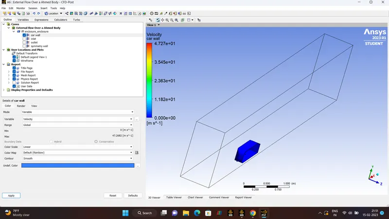
Velocity Contour.

 

RESIDUALS.

 

DRAG CO-EFFICIENT.

 

LIFT CO-EFFICIENT.

 

DRAG AND LIFT RESULTS.

CFD-POST.

PRESSURE and VELOCITY.

  

VELOCITY VECTOR.  

 

 

 

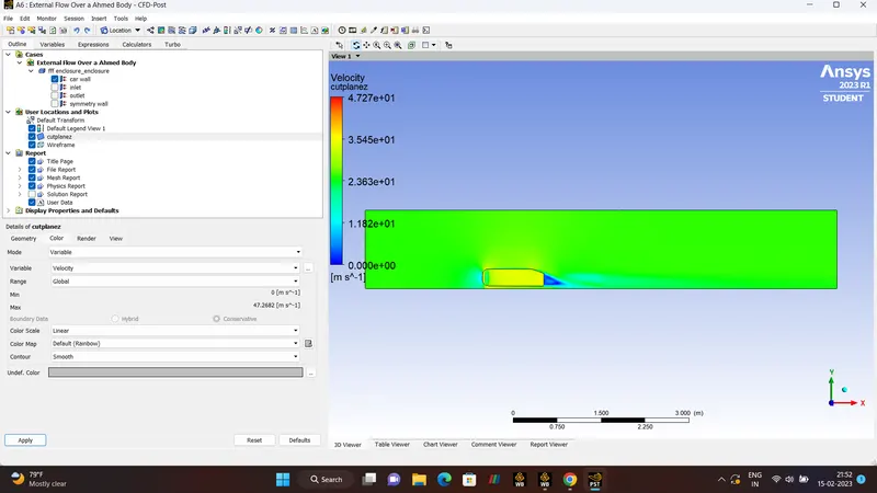
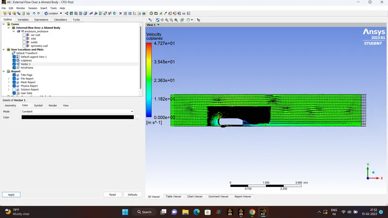
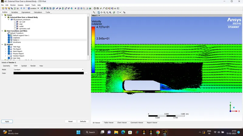
RESULTS OF VELOCITY u.

PRESSURE VECTOR.

 

ANIMATION OF VELOCITY MAGNITUDE. 

GRID INDEPENDENCE TEST. 

NO	Turbulence Model	Number of Element Size	Number Of Iterations	Drag Co-efficient (cd)	Lift Co-efficient (cl)
1	K-epislon	94192	1000	0.34	0.26
2	K-omega	357630	700	0.29	0.21
3	K-epsilon	316797	500	0.32	0.27

 

• CONCLUSION:-

Let us conclude that the Grid independence is performed and the values of the drag and lift co-efficient is done.

We can conclude that the Vector plot is clearly shown in the CFD-POST in the rear end of the ahmed body.

Hence the velocity and Pressure magnitude is evaluvated and there is a negative pressure in the wake region because there no flow in that particular area as pressure decreases.

We can perform both in the Laminar and turbulence flow, in our case turbulence is choosen and the grid independence is done with both models( Omega and Epsilon).