External flow simulation over an Ahmed body using ANSYS Fluent
Week 3 Report
- Aim: To understand the behavior of the Ahmed Body and perform an External Flow simulation on a given model.
- Theoretical Introduction:
The Ahmed body is a simplified car body used in the automotive field to study the impact of the flow pattern on the drag. The external aerodynamics of the car defines many major traits of an automobile like stability, comfort, and fuel consumption at high speeds. The flow around the vehicle is characterized by high turbulent and three-dimensional flow separations as well as there is a growing need for more insight into the physical features of these dynamical flows. The Ahmed Body is a simplified car, used in the automotive field to investigate the flow analysis and find the wake flow around the body. Ahmed body is made up of around the front part, a moveable z slant plane in the rear of the body to study the detachment phenomena at different angles, and a rectangular box that links the front part and the rear slant plane. The principal objective to study such a simplified car body is to tackle the flow processes involved in drag production. Through perceiving the mechanisms involved in creating drag one can be able to design a car to minimize drag and therefore reducing fuel consumption and maximize vehicle performance.
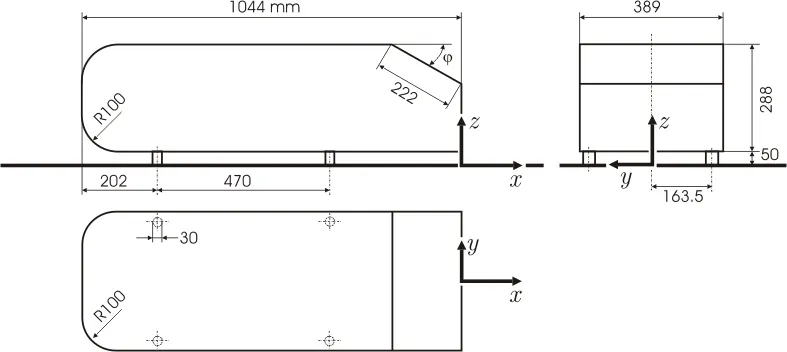
Geometry of an Ahmed Body
The “Ahmed” body, has the form of a highly simplified car, consisting of a blunt nose with rounded edges fixed onto a box-like middle section and a rear end that has an upper slanted surface (like a “hatch-back” car), the angle of which can be varied. The model is supported on circular-sectioned legs or stilts, rather than wheels. Despite neglecting a number of features of a real car (rotating wheels, rough underside, surface projections, etc.) the Ahmed body generates the essential features of flow around a car, namely: flow impingement and displacement around the nose, relatively uniform flow around the middle and flow separation and wake generation at the rear.
Besides the analyses of the velocity field, the Ahmed Body is also used for drag force and lift force analyses and rolling, pitching, and yawing moments. The slant angle on the back allows studying the separation region and its influence on the velocity profile and forces.
The geometry of the Ahmed body is shown in the figure below. The slant angle is adjustable and is the main variable model parameter in the experimental investigations. The Ahmed body, of length (L) 1044 mm, height (H) 288 mm, and width (W) 389 mm, was placed at 50 mm from the ground (G).
- Questions:
Q. Describe Ahmed's body and its importance.
Ans. Ahmed Body is a simplified body of a car that can be used to validate and calibrate the different CFD Softwares that are being built. It is basically used to validate if the code running behind in the solver is written correctly or within a certain percentage of error.
Q. Explain the reason for the negative pressure in the wake region and Point of Separation.
Ans. The flow around the Ahmed reference body is complicated. Due to the slant in the rear of the vehicle, flow separation and counter-rotating vortices are generated at the slant edges. The drag forces of Ahmed Body reach a maximum when the slant angle is 30 deg. For slant angles higher than this value, the adverse pressure gradient in between the slant and the roof is so intense that the flow fully detaches over the slant. Below these critical slant angles (30 degrees), the flow still separates but the pressure difference between the slant region and the side walls is still sturdy enough to generate substantial stream-wise vortices at the lateral slant edges. These prompt a downward motion over the slant, mainly in the downstream part. As a result, the flow separates at the upstream end of the slant can couple further to the downstream. The flow around the Ahmed body has several flow separations from the front to the rear of the vehicle. The flow recirculation caused by these flow detachments contributes to the vehicle’s drag. The location point at which the flow separates determines the size of the separation zone, and accordingly the drag force, thus an exact simulation of the wake flow and of the separation process is essential for the accurate result of drag predictions.
Negative pressure gradient
When fluid velocity increases, the pressure decrease. The wake region is formed due to adverse pressure in the rear end causes the boundary layer to separate out from the body. The wall shear stress and velocity become zero and wake formation starts. These wakes are nothing but small vortices that create negative pressure. These create a circulation of velocity and induces drag forces.
Point of separation
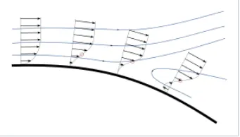
Separation occurs due to an adverse pressure gradient encountered as the flow expands, causing an extended region of separated flow. The part of the flow that separates the recirculating flow and the flow through the central region is called the dividing streamline. The point where the dividing streamline attaches to the wall again is called the reattachment point. As the flow goes farther downstream it eventually achieves an equilibrium state and has no reverse flow. When the boundary layer separates, its remnants form a shear layer and the presence of a separated flow region between the shear layer and surface modifies the outside potential flow and pressure field. In the case of airfoils, the pressure field modification results in an increase in pressure drag.
- Procedure:
1. We begin the procedure to work on the Ahmed Body in the Space-Claim tool of the ANSYS Workbench. Here we will cut the Ahmed body at the global origin and then use the split body command to split the Ahmed Body into two halves so that we reduce the number of cells for the simulation. This will help us fasten the entire simulation while maintaining the same level of accuracy as the solver then considers both the sides of the Ahmed body with the names that we give as the Boundary Conditions of the Walls of the Ahmed Body.
2. There are various cases that we need to study. Firstly we create an enclosure around the Ahmed Body. We then go onto meshing this case set up and then use it for this case.
The outer enclosure was created as follows: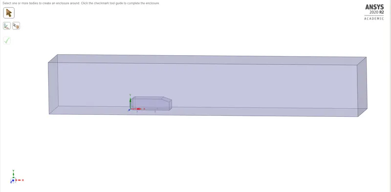
- The right face is located at a distance of 5m from the right side face of Ahmed body along the X-axis.
- The left face is located at a distance of 2m from the left side face of Ahmed body along the X-axis.
- The top face of the encloser is at a distance of 1 m from the top side face of the Ahmed body along the Y-axis.
- The bottom face of the encloser is attached to the bottom face of the Ahmed body along the YZ plane.
- The front and back face of the encloser is at a distance of 0.5 m along the Z-axis.
3. In the next step, we will generate the Mesh for the Outer Enclosure.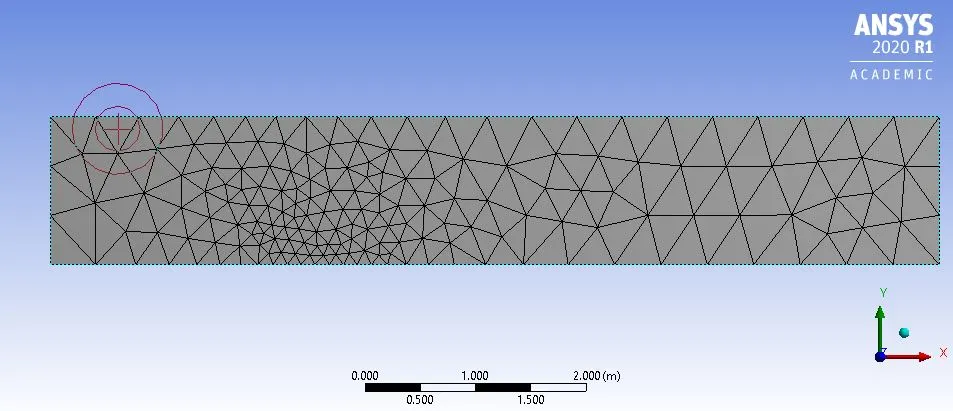
We use the Mesh Tool in the Ansys Workbench and then mesh the base setup that we have. The mesh size is 0.35m as the average size of the mesh.
4. We are using the K-E model (K-Epsilon) as viscous property and taking the initial Velocity as 25m/s. Pressure-based solver and steady-state simulation are to be generated, We are going to observe the Velocity & Pressure contours to estimate the results and which can be useful in further future modification.
5. We have to simulate this as the first case and then in the next case we create another smaller enclosure around the Ahmed Body which we will then later edit for the purpose of Mesh Refinement. The Inner Enclosure was created as follows:
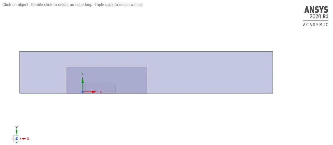
- The right-hand side of the face is located at a distance of 1 m from the right side face of Ahmed body along the global X-axis.
- The left face hand side of the face is located at a distance of 0.5 m from the left side face of Ahmed body along the global X-axis.
- The top face of the encloser is at a distance of 0.5m from the top side face of the Ahmed body along the global Y-axis.
- The bottom face of the encloser is attached to the bottom face of the Ahmed body along the YZ plane.
- The front and back faces of the encloser is at a distance of 0.26 m along the global Z-axis.
6. Another Important Step that we must do is the Interference clearing between the two enclosures that we have created.
As we know, initially there was a huge interference between the Outer and Inner encloser so that the mesh gets overlapped which gets not acceptable so to avoid this we made share topology and get deleted the Interference region that by using the interference command after this we get a good interaction between the Inner and Outer enclosers so that we can get the mesh properly and also share the boundaries between them. The following image shows: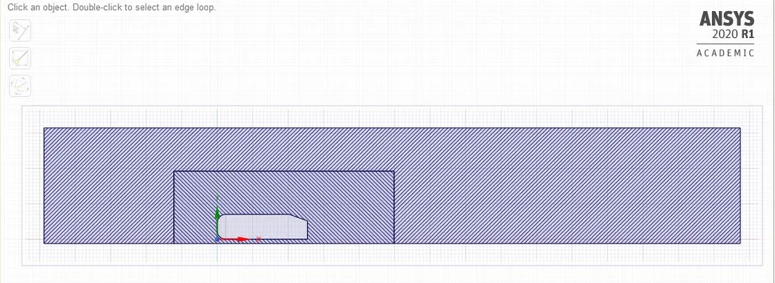
After Clearing all the Interference in the model.
7. When we have to refine the mesh of the outer enclosure, we must perform a Hexa Mesh over it.
In this meshing, we can assign the named selection for Inlet, Outlet, Symmetry wall, and Car Wall, We can use the different types of meshing processes for this model.
In this we follow three stages, Meshing will be done for the outer enclosure chosen as a method of the Multizone and this will create the Hexa mesh, The element size used for this is 0.08m.
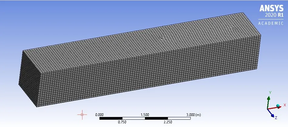
Outer Enclosure Meshed.Next for the inner enclosure, we choose the body sizing method to make more refinement, the element size we use for this is 0.04m.
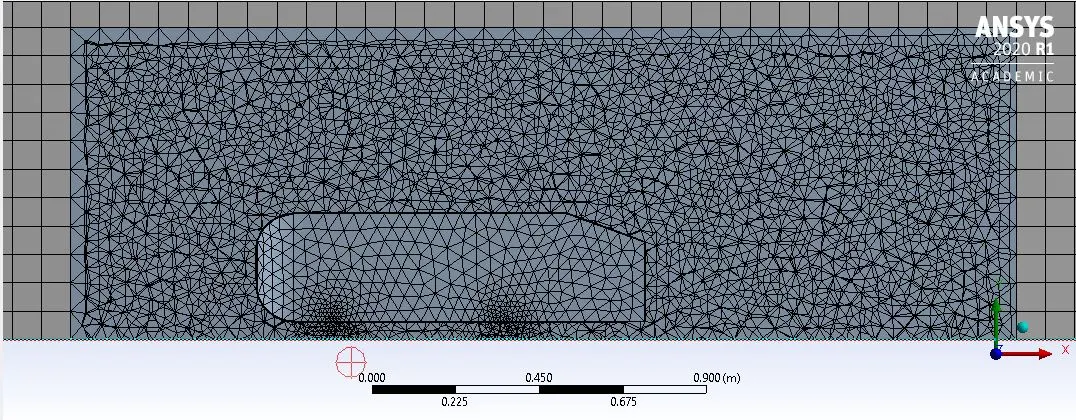
Mesh around the Ahmed BodyNext, we select the face sizing method to select the legs of the body to capture them with better refinement, we take the element length as 0.005m.
Next, to capture the flow over the body we make the inflation layer which helps us in capturing the flow very finer way and the mesh will also be capture along the body perfectly. We take the number of inflation layers as 6, Total thickness value as 0.0036.
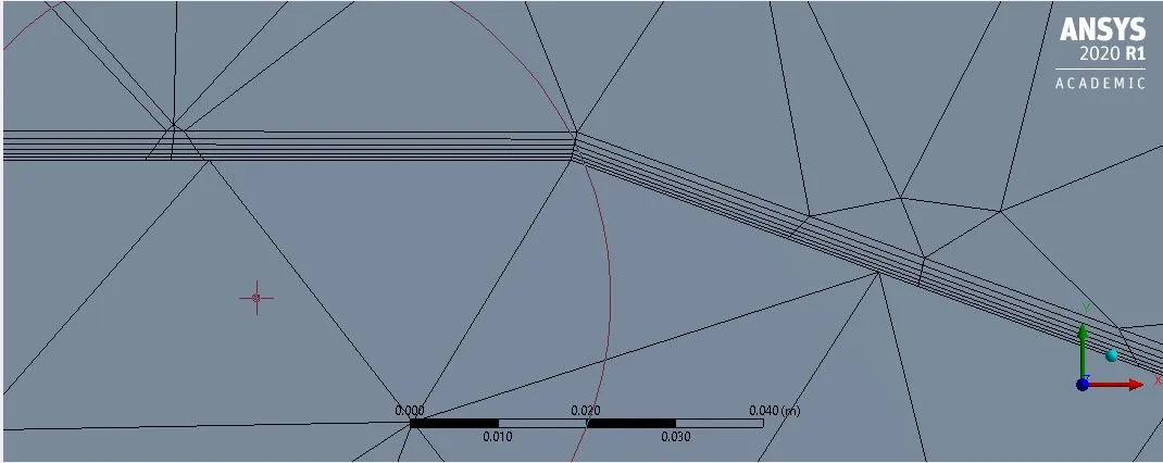
Inflation Layer Added.
8. Solver type: Pressure based
Check the Energy equation
Turblent Model: K-Omega SST model
Fluid Material: Air
Boundary conditions
Inlet velocity : 25 m/s
Outlet pressure : 0 pa
Symmetry: For sidewalls
Wall: Bottom,
Creating a surface plane to observe the contours.
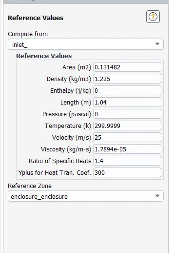
Reference Values - Results:
1. The first case that we performed the setup for is with a mesh size of 0.35m.
We get the following plots: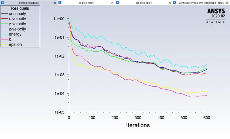
Scaled residuals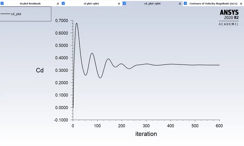
Coefficient of Drag plot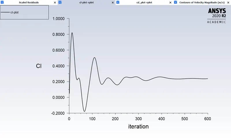
Coefficient of Lift Plot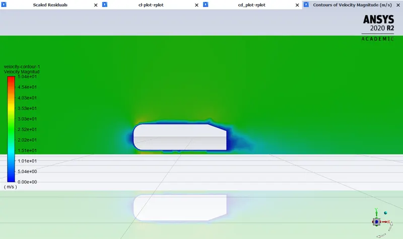
Velocity contour showing the Wake region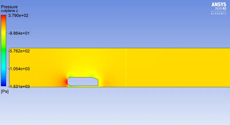
Pressure Contour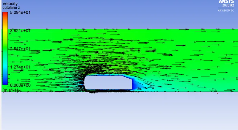
Vector plot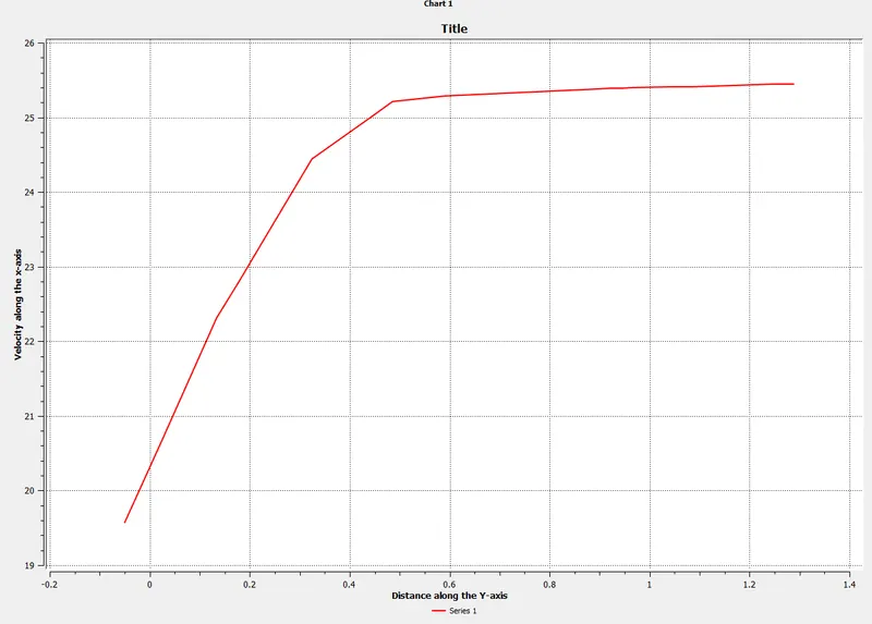
Velocity Plot
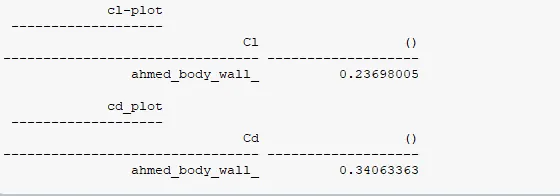
Values of Coefficient of Drag and Lift
2. In the second case we can see and observe the grid dependency and to understand this, we simply change the mesh size around the Ahmed Body. Soo, we have done two more simulations with two different sizes of Mesh.
2.a. Mesh size = 0.03m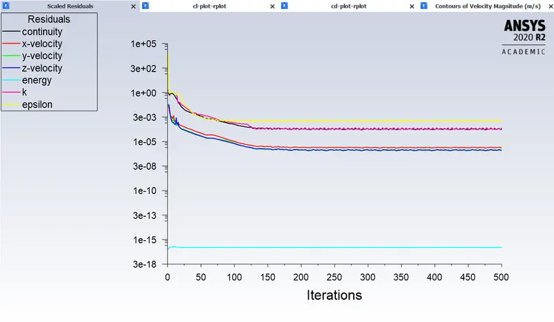
Scaled Residuals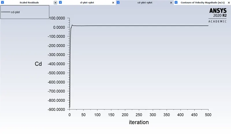
Coefficient of Drag Plot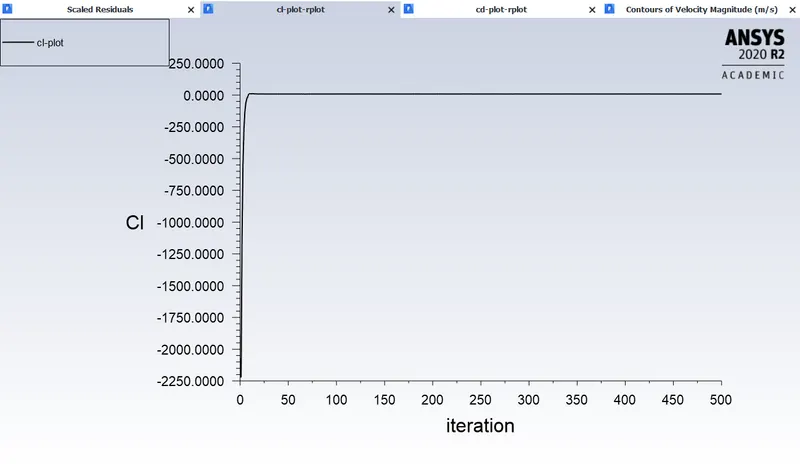
Coefficient of Lift Plot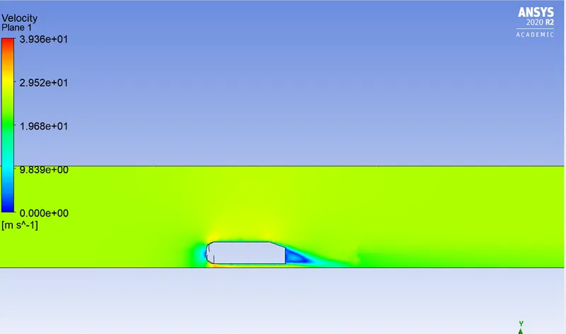
Velocity Contour showing the wake region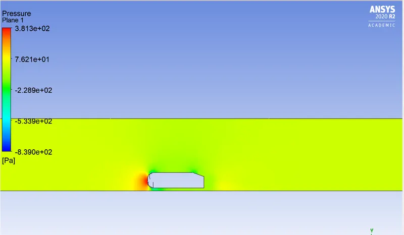
Pressure Contour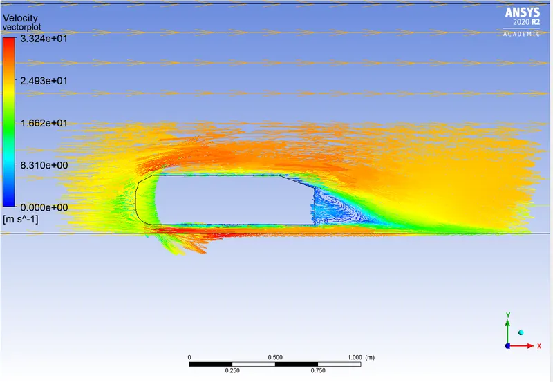
Velocity Vector Plot showing the wake region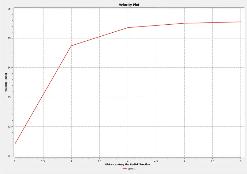
Velocity Plot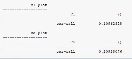
Values of Coefficient of Drag and Lift
2.b. Mesh Size = 0.2m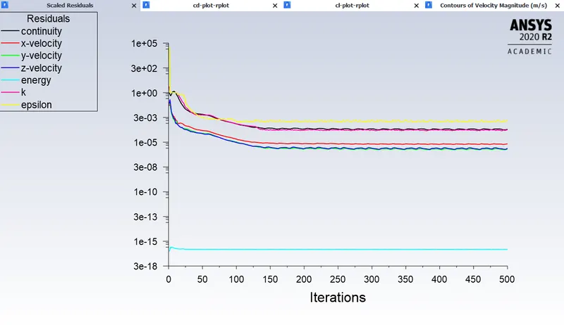
Scaled Residuals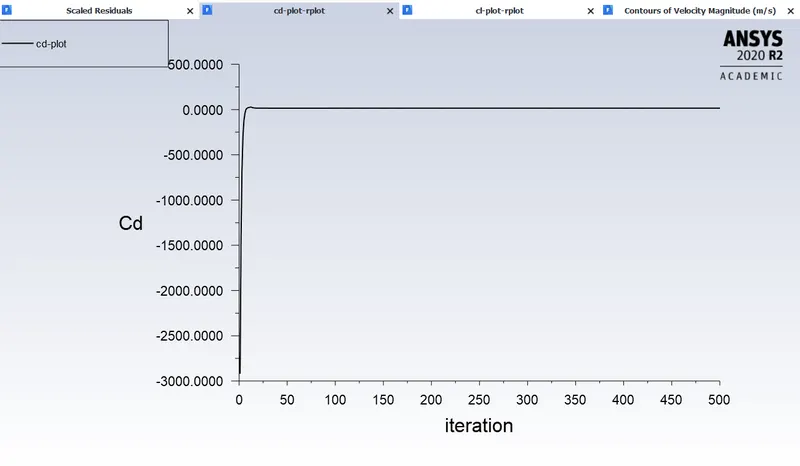
Coefficient of Drag Plot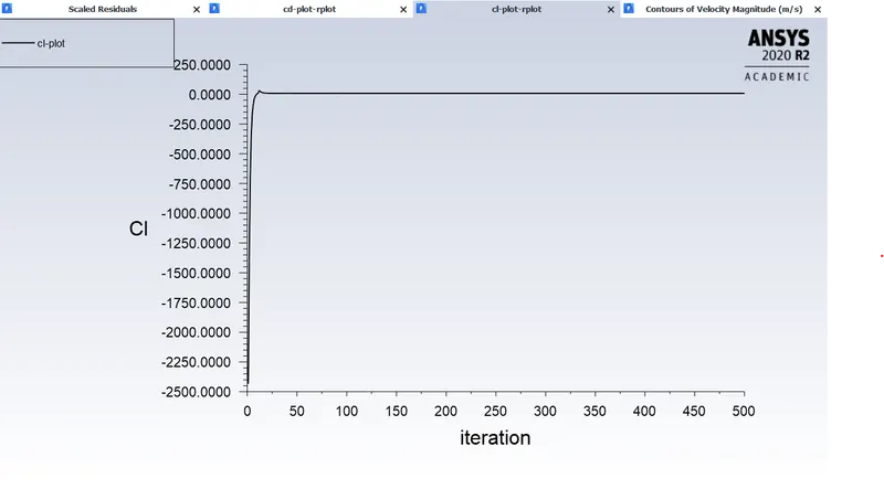
Coefficient of Lift Plot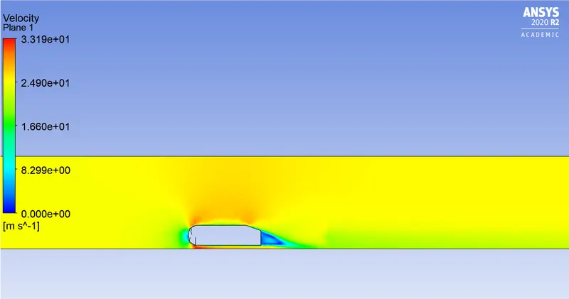
Velocity Contour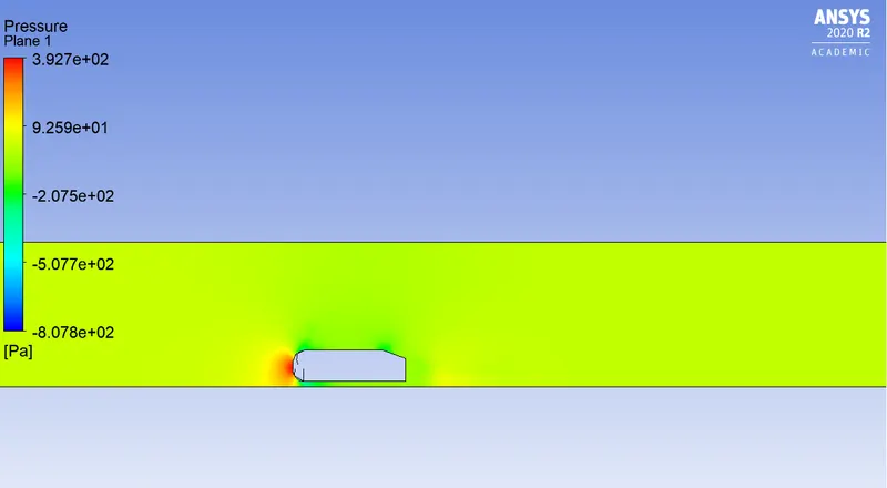
Pressure Contour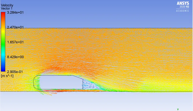
Velocity Vector Plot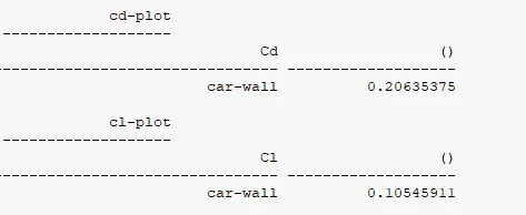
Values of Coefficient of Drag and Lift - Conclusions:
1. We understand that the baseline simulation has also given us a not very accurate answer for the conditions at which we are currently simulating the Ahmed body model.
2. As we refine the mesh and make it much finer, we observe that we get much more accurate results.
3. We even studied the effects of different mesh sizes on the model and can conclude that the physics of the problem does not change but if there is quite a significant change in the Mesh size, the accuracy of the simulation will change.