Week 3 - External flow simulation over an Ahmed body.

WEEK 3: SIMULATION OF EXTERNAL FLOW OVER AHMED BODY

AIM:

To perform grid independence study for flow over Ahmed body and compare the drag coefficients for each case.

THEORY:

Ahmed body and its application:

Ahmed body is a condensed model representation of actual passenger vehicle which was proposed by Ahmed in 1984 to study the geometric effects on the wakes of ground vehicles. Ahmed body is used to capture the flow features around the body which can be observed in case of an original automobile. The study of such simplified body helps us to determine the flow patterns which induces drag component around the body. Following corrective measures, one can analyse the factors that can minimize drag and therefore improve vehicle performance. It is also used to validate or verify the CFD codes.

PROCEDURE:

CASE 1 Baseline simulation:

The base line simulation is concerned with running the simulation with default mesh assigned to the body and based on the results of the simulation further corrections are made to obtain the required results.

GEOMETRY SETUP:

• Import the ‘Ahmed body’ model in to the Space Claim interface.
• 
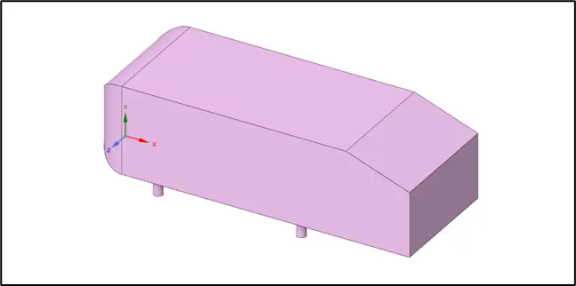
• Prepare an enclosure around the body for CFD analysis.
• 
• 
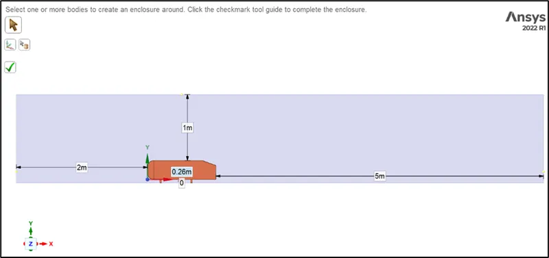
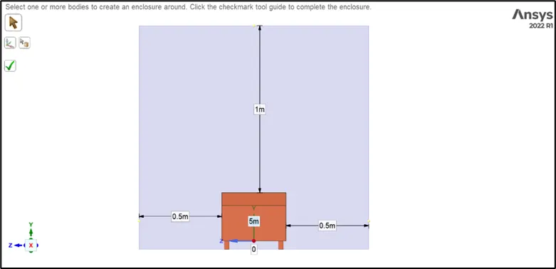
• Since the entire setup is symmetric, the simulation can be made easier by considering only on half of the setup.
• Insert planes by selecting origin and enable the ‘XY’ plane. Use ‘split body’ option to remove one half of the setup.
• 
• 
• 
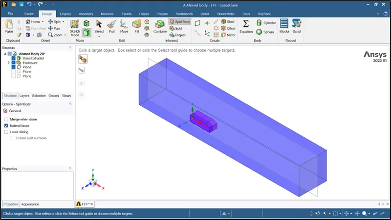
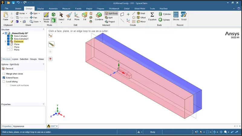
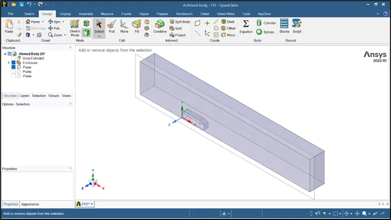
• Supress the Ahmed body (Boss-Extrude2) for further analysis.
• Enabling ‘cut view’, it can be observed that the hatch pattern around the Ahmed body is uniform and this will help to capture a proper mesh.
• 

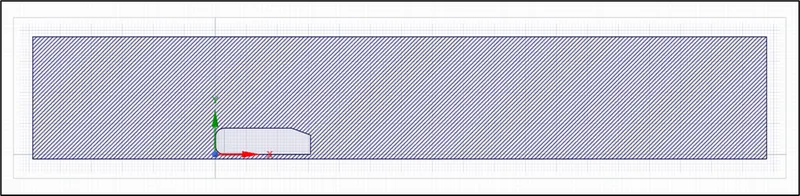
MESHING

• Double click on ‘ANSYS Mesher’ to load the geometry to mesh interface.
• Click on ‘generate mesh’ to assign default mesh to the model.
• The model contains 42964 elements for a mesh element size of 409.2 mm triangular elements.
• 
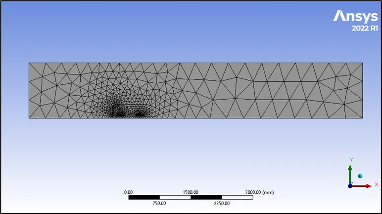
• Assign the named selections.
• 
• 
• 
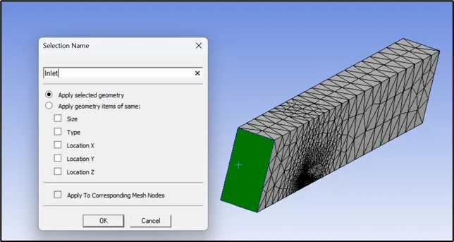
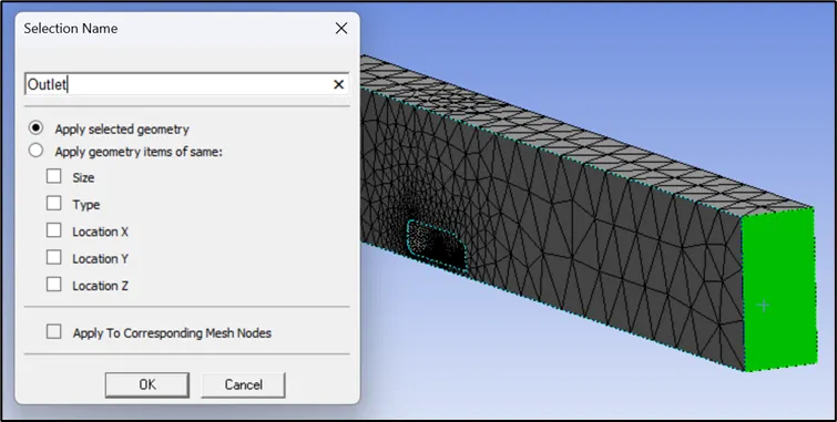
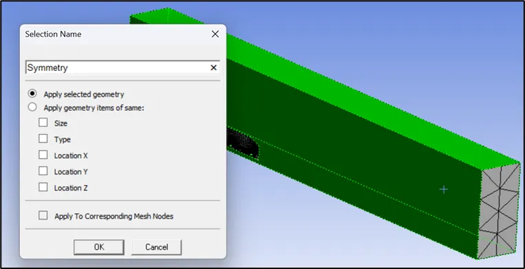
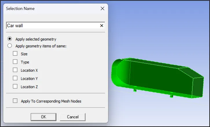
• Hide all the faces of the enclosure and using ‘box select’ option select the Ahmed body and assign it as car wall.
• 

SIMULATION SETUP:

• Given velocity as 25 m/s, the Mach number can be calculated as,

• Since the Mach number is less than 0.3, we can consider the pressure based steady state solver.
• 
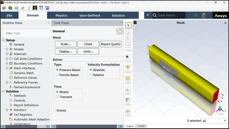
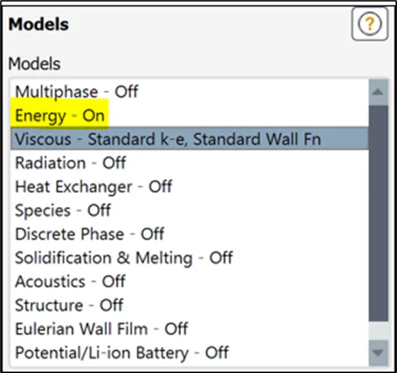
• Select ‘k-epsilon’ turbulence model and select enable ‘energy.’
• 
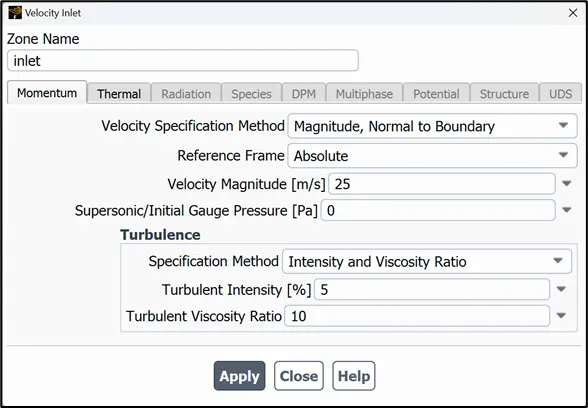
• Set the material and boundary conditions default except for inlet, which is specified as 25 m/s.
• 
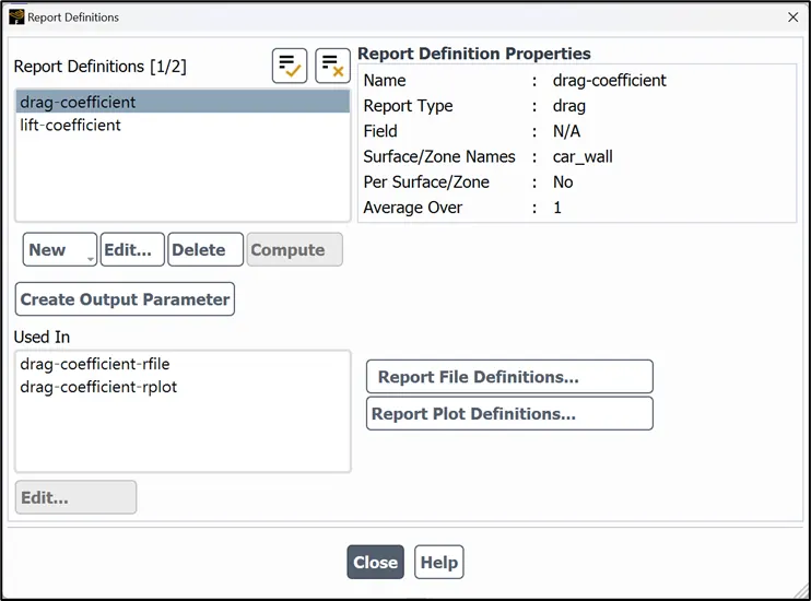
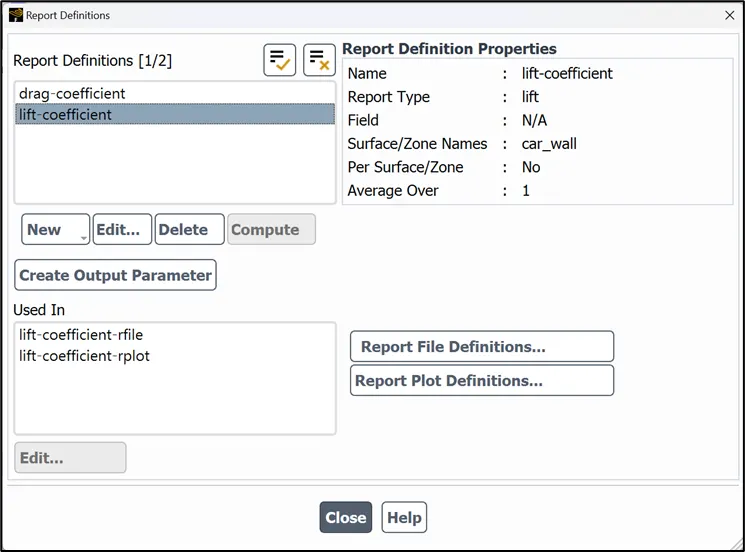
• Define reports for drag and lift coefficients.
• 
• 
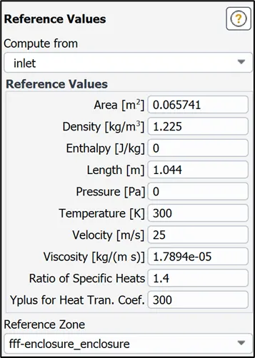
• Select the reference values to be calculated from inlet.
• 
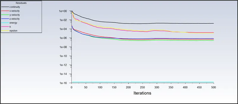
• Initialize the solution using ‘hybrid initialization’ and run the simulation for 500 iterations.

Residual plot

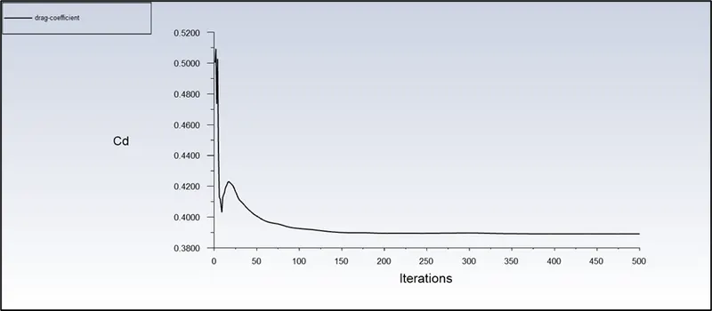
Drag coefficient plot = 0.389114

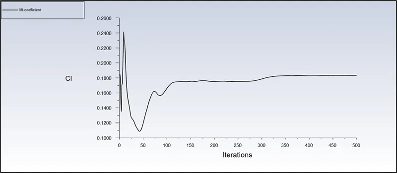
Lift coefficient plot = 0.183067

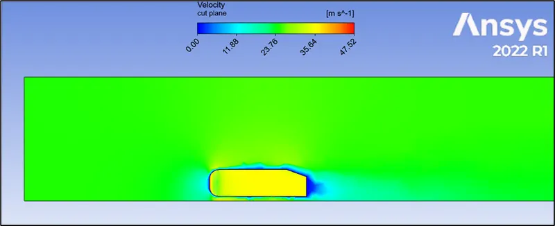
Velocity contour

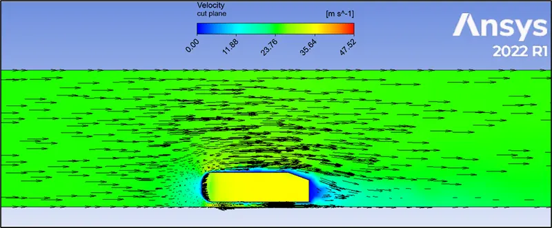
Velocity vector plot

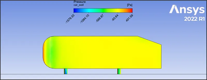
Pressure contour for car wall

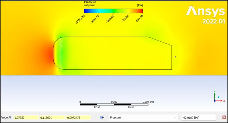
Pressure contour at XY cut plane

Observations:

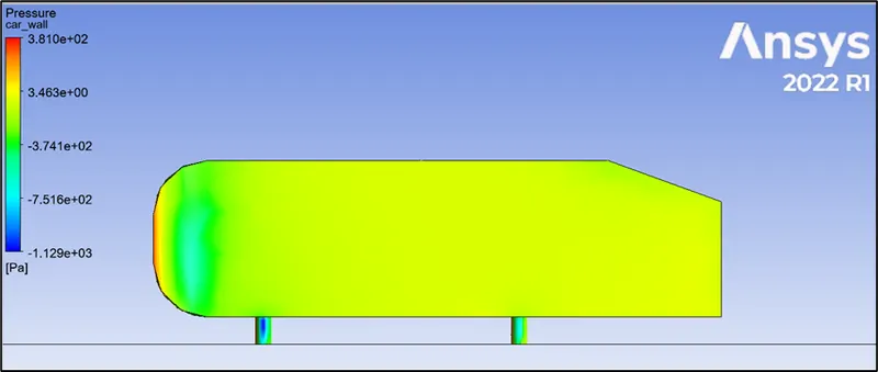
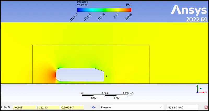
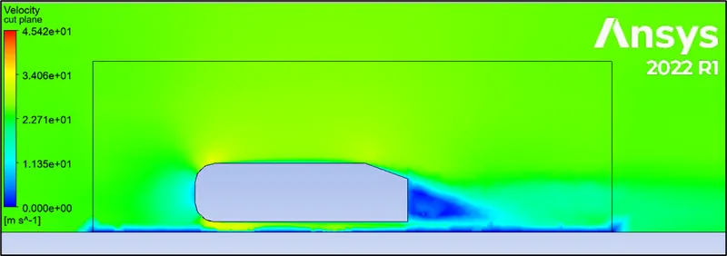
• The velocity plot obtained shows a coarse wake region formed at the rear end of the Ahmed body. The pressure is also observed to be attaining negative value as we move away from the front end (pressure plot) which is due to the pressure drag produced during flow separation occurring at the slant edges of the body. The point at which the separation occurs is the ‘point of separation.’
• The location of this point determines the area of separation, which contributes to the drag force. The drag force will be higher as the area of separation increases causing low pressure wake region which hampers the overall vehicle performance.
• As observed from the vector plot, the aim is to obtain a wake region with reduced the drag force to improve the vehicle performance. This can be done by reducing the mesh element size, changing the mesh element type and adding inflation layers around the body to capture the flow more accurately.

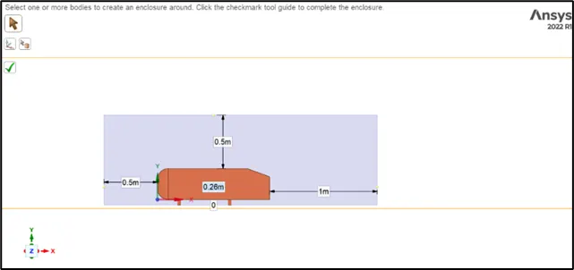
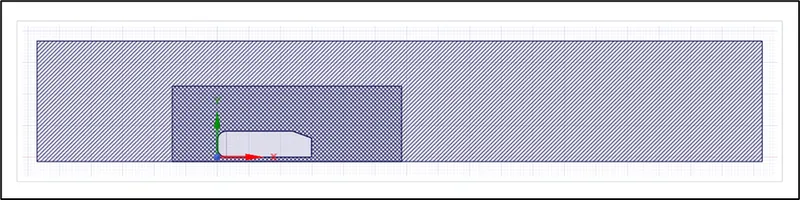
• Before proceeding with mesh refinement, we can add another enclosure with dimensions as shown in figure.
• 
• 
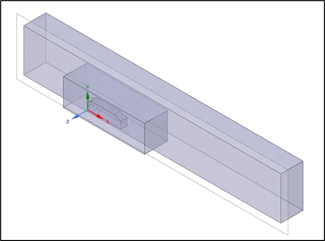
• Use ‘split body’ command to delete one half of the enclosure.
• 
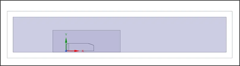
• Select the XY plane and click on cut option to view the interference pattern of both enclosures.
• 
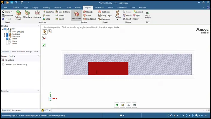
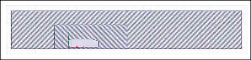
• The interference is resolved using the ‘interference’ option.
• 
• 

CASE 2.

Outer enclosure = 100mm, inner enclosure = 50mm, face sizing = 5mm

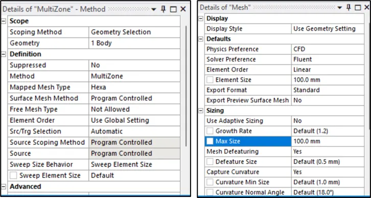
• To obtain the maximum mesh efficiency, the enclosure can be meshed with Hexa elements by adding a ‘multizone’ method.
• Set the element size and the maximum element size as 100 mm and generate mesh.
• 
• 
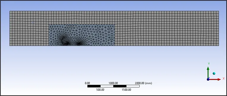
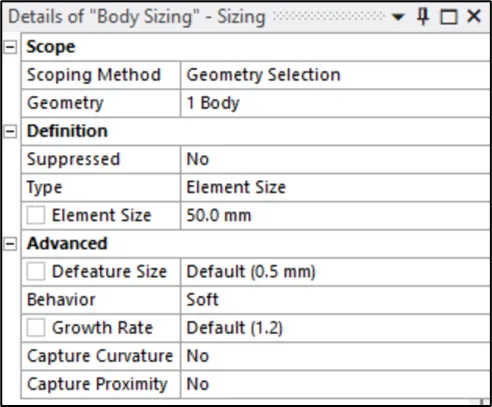
• Next step is to add inflation layers around the Ahmed body, which is done by inserting a sizing on the inner enclosure and set the element size as 50 mm.
• 
• The zoomed view at the bottom face shows that there is polygonal profile for holes which is to be refined.
• 
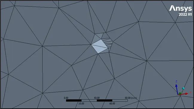
• Insert a sizing for the cylindrical surface and set the element size as 5 mm.
• 
• 
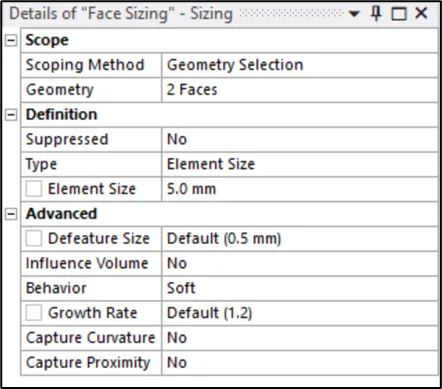
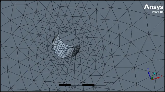
• Next step is to insert the inflation layers around the Ahmed body.
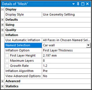
• Click on mesh and under ‘inflation’ option select ‘all faces in chosen named selections’ and select ‘car wall’ in name selection.
• Since it is turbulent flow, the Y+ can be considered as 150, (30 -300 for a turbulent region) and based on that the first layer thickness is calculated as 2.197 mm.
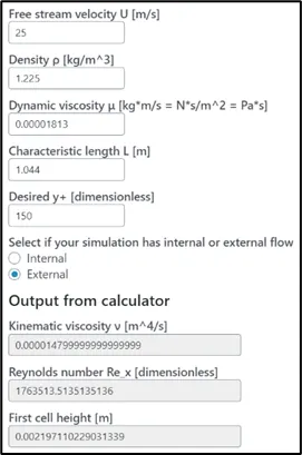• Source: Volupe Engineering software Y+ calculator
• The maximum layers are set as 8 with a growth rate of 1.2.
• 
• Click on generate mesh.
• 
• 
• 
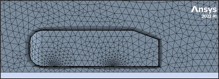
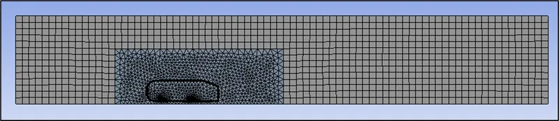
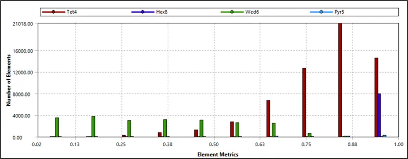
• The refined mesh shows a total number of 90393 elements with an average element quality of 0.708.

Residual plot

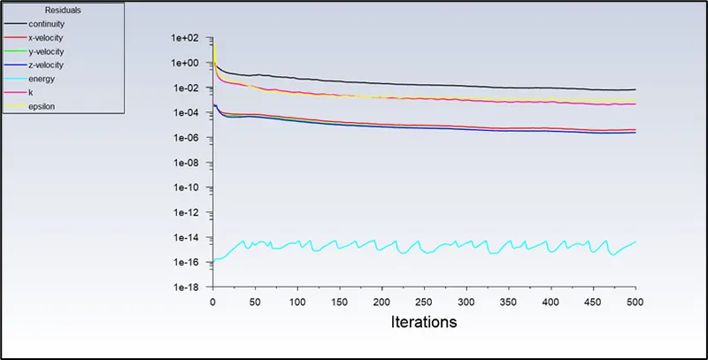
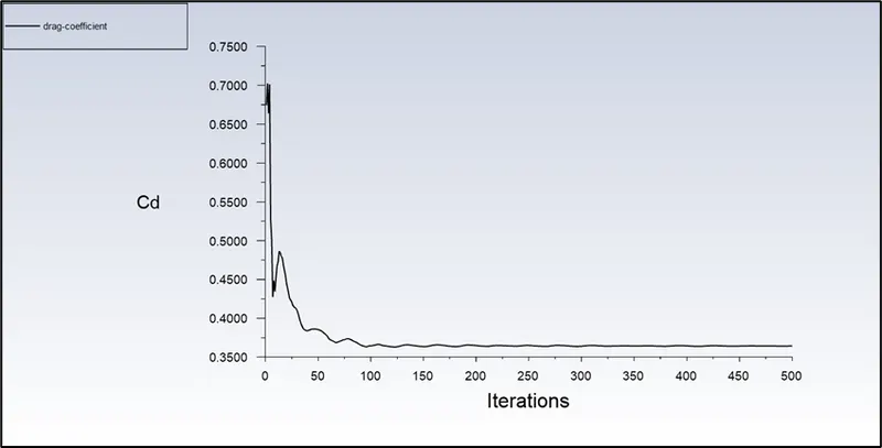
Drag coefficient plot = 0.36443

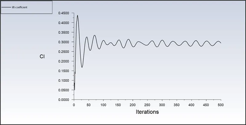
Lift coefficient plot = 0.29314

Pressure contour at car wall

Pressure contour at XY cut plane

Velocity contour

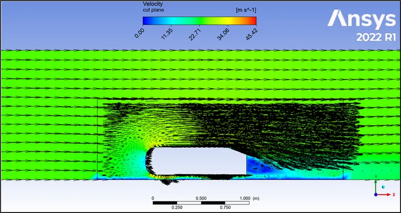
Velocity vector

Observations:

The drag is significantly reduced to 0.36443 and the flow is better captured at the wake region after mesh refinement. The decrease in the drag coefficient can be associated with the presence of a boundary layer attached to the car wall.

CASE 3.

Outer enclosure = 50mm, inner enclosure = 25mm, face sizing = 3mm

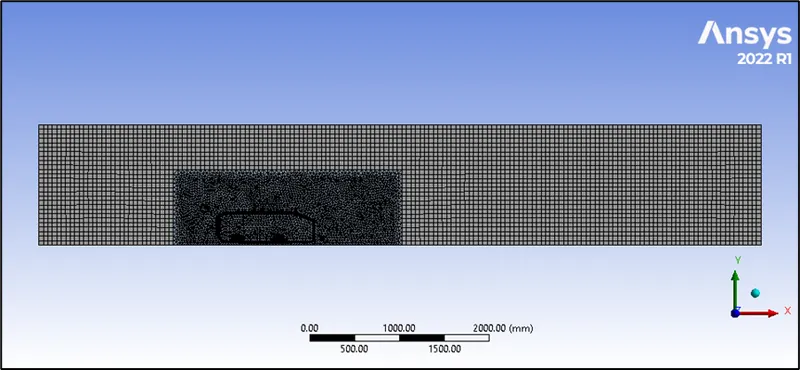
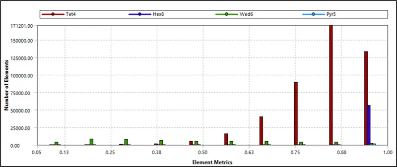
• The total number of elements are 564355 with an average element quality of 0.817.

Residual plot

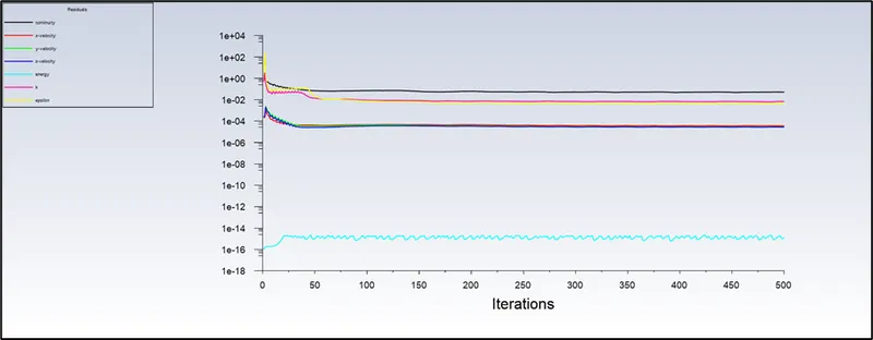
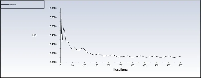
Drag coefficient plot = 0.33164

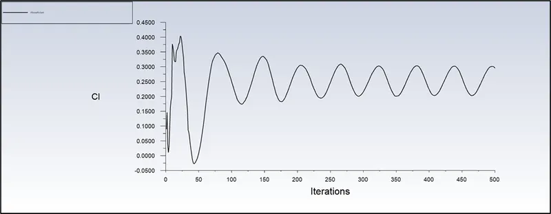
Lift coefficient plot = 0.29542

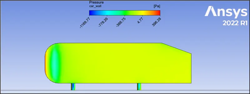
Pressure contour at car wall

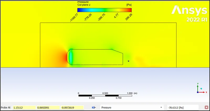
Pressure contour at XY cut plane

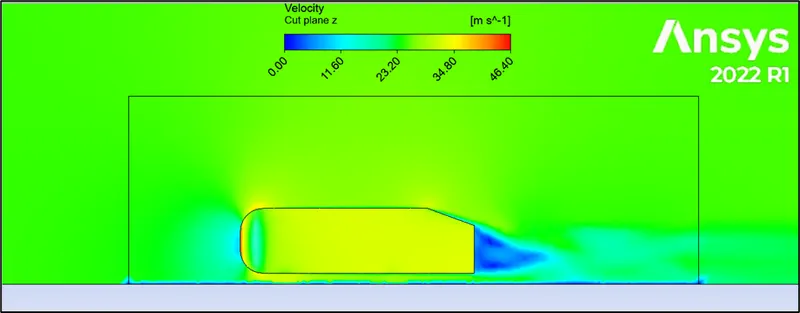
Velocity contour

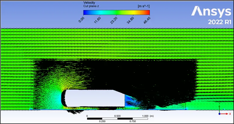
Velocity vector

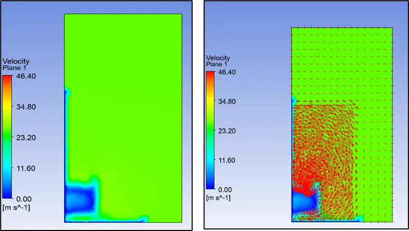
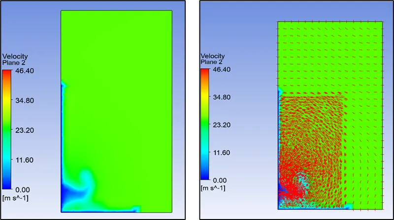
Further, for refined mesh case the vectors are created in YZ plane at 1.1m, 1.3m and 1.5 m.

Velocity contour and vector plot at 1.1m YZ plane

Velocity contour and vector plot at 1.3m YZ plane

Velocity contour and vector plot at 1.5m YZ plane

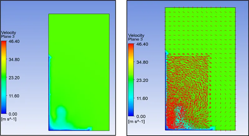
Observations:

• The drag coefficient is further reduced to 0.33164 and the wake region is captured more accurately due to fine meshing. Also, the velocity and velocity vector plots at different cross sections taken show the formation of a counter rotating vortex (only one side of vortex shown).
• Initially, there is a presence of slight recirculation near the slant end of the Ahmed body which signifies the presence of boundary layer separation. Further, as we move away from the slant region the recirculation region starts diminishing and this can be inferred as the flow has reattached itself leading to a circulation region at the lower end of Ahmed body.

COMPARISON OF RESULTS AND CONCLUSION

	Base line mesh	Case 1	Case 2
Outer enclosure (mm)	409.2	100	50
Inner enclosure (mm)	-	50	25
Face sizing (mm)	-	5	3
Inflation (first layer thickness in mm)	-	2.197 with 8 layers
Number of elements	42964	90393	564355
Average element quality	0.829	0.708	0.817
Drag coefficient	0.389114	0.36443	0.33164
Error % in drag coefficient	15	9.4	0.49
Lift coefficient	0.183067	0.29314	0.29542

• Thegrid independence study for external flow over Ahmed body is performned and the refined mesh has produced the best drag coefficient result of 0.33164 with an error of 0.49% which are is accord with the required drag coefficient value of 0.33.
• The velocity flow is better captured with mesh refinement which has reduced the drag coefficient significantly in comparison with the default meshing case.