Week 3 - External flow simulation over an Ahmed body.

Aim: To perform the external flow simulation over Ahmed's body.

Objective:

1. To determine the aerodynamic forces on the Ahmed body such as drag and lift coefficient. 
2. To perform the grid dependency test.

Introduction: 

Ahmed body:  

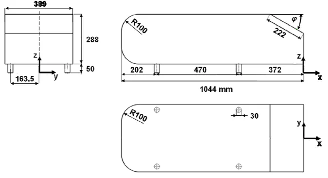
• The Ahmed body is a generic car body (a simplified vehicle model). The airflow around the Ahmed body captures the essential flow features around an automobile and was first defined and characterized in the experimental work of SR Ahmed in his research Some salient features of time average ground vehicle wake. Although it has a very simple shape, the Ahmed body allows us to capture characteristic features that are relevant to bodies in the automobile industry.
• This model is also used to describe the turbulent flow field around a car-like geometry. Once the numerical model is invalidated, it is used to design new models of the car. The rear part of Ahmed's body called as 'slant angle' which influences drag and lift with its critical slant angle which is around 0-30 degrees.
• It is used for testing new CFD solvers or testing one's ability to perform simulations as there is a plethora of experimental data available about the Ahmed body to compare simulation data to.
• In this project, I will be performing analysis on an Ahmed Body in ANSYS using the Fluent solver.

Importance of Ahmed's Body:

• Ahmed's Body plays a vital role in testing the aerodynamic properties of vehicles.
• It is also used to describe the turbulent flow field around a car-like geometry and later to design new car models with validated results.

Theory:

1) Y+ Concept:

When any viscous flow flows over a surface, a region of slow-moving flow called the boundary layer develops. Inside the boundary layer, there is a strong velocity gradient and U varies non-linearly. It is important to distinguish these layers to model the boundary physics correctly and use an appropriate turbulence model. Hence, Y+ is a non-dimensional distance normal from the wall. It is applicable to all flows. For a CFD simulation, we can compute the first layer height for a desired Y+ value with the following formula:

  

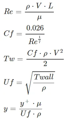
Where,

ρ is fluid density ;

µ  is fluid viscosity ;

U is the free stream velocity ;

L is characteristic length ;

U_τ  is frictional velocity ;

τ_ω is wall stress ;

C_f is the skin friction coefficient 

2) Boundary Layer:

The boundary layer is a thin layer of a real fluid along the surface of an object in which viscosity affects fluid dynamics. When fluid flows over a plate, velocity near the surface is much lower and vorticity is present. The no-slip condition accounts for zero relative velocity at the plate and keeps on increasing until it reaches the free stream velocity. The thickness of the boundary layer increases along the length of the plate. In a narrow boundary layer adjacent to the plate, the shear forces and inertia forces are equally important in determining the motion of the fluid element and outside of the region, shear stresses can be neglected. The fluid deceleration is transferred from one fluid layer to another fluid layer by viscosity and it forms the velocity gradient in the boundary layer. The thickness of the boundary layer is often described as the distance from the plate until the velocity reaches 99 % of the free stream velocity.

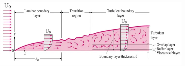
The gradient of the velocity normal to the wall (∂u/∂y) times the viscosity (μ) is the wall skin friction or shear stress. The greater the velocity gradient normal the wall, the greater the shear stress. As the velocity gradient goes on decreasing along the flow direction, the shear stress also decreases. The growth of the boundary layer thickness along the plate can be explained by considering the time history of the vorticity within the boundary layer. The viscosity acts through the mechanism of molecular diffusion to spread out the vorticity as it is convected downstream. The local boundary layer thickness is the measure of the distance for vorticity diffused away from the plate.
Since we are dealing with the turbulent boundary layer and related phenomena, let us not get into the laminar boundary layer. From the above figure, it can be seen that in the turbulent boundary layer region flow near the wall has been analyzed in terms of three layers. The inner layer, or sublayer (where viscous shear dominates), The outer layer or defect layer (where large-scale turbulent eddy shear dominates), The overlap layer or log layer (where velocity profiles exhibit a logarithmic variation)

3) Flow Separation:

When a fluid is forced to flow over a curved surface at high velocities. A fluid follows the front portion of the curved surface with no problem, but it has difficulty remaining attached to the surface on the backside. At sufficiently high velocities, the fluid stream detaches itself from the surface of the body. This is called flow separation. The location of the separation point depends on several factors such as the Reynolds number, the surface roughness, and the level of fluctuations in the free stream, and it is usually difficult to predict exactly where separation will occur unless there are sharp corners or abrupt changes in the shape of the solid surface. This contributes to the formation of pressure drag which affects the vehicle's performance.

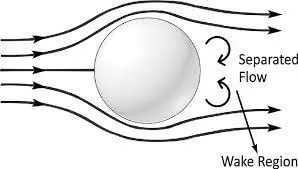
When the vehicle is moving at a certain velocity the fluid imparts viscous force to the vehicle as long as it is in the viscous sublayer of the boundary. When the fluid reaches the rear end of the vehicle it gets detached from the surface of the body causing negative pressure in the wake region. The movement of the fluid around the vehicles depends on the geometry of the car and the Reynolds number.

When the flow is attached to the body of the vehicle the viscous force will increase which will increase the pressure and decrease in velocity before the rear end of the vehicle. As soon as the air encounters the sharp turn causing the velocity decreases resulting in the negative pressure region which is in the wake region. The recirculation region happens beyond the point of separation.

If the rate of change of pressure is large the mixing process will not occur and the boundary layer flow stops. The above figure shows that at the point of turning the flow gets separated from the boundary layer and there is a region of recirculation after which the flow attaches itself to the boundary layer. In order to reduce the separation of fluid from the boundary layer, it is advisable to have a smooth edge to reduce the effect of drag on the vehicle.

Solving & Modeling approach:

1) Baseline simulation approach using k-ε">k-ε model.

• Ahmed's body is loaded into the Spaceclaim.
• A single enclosure is drawn across Ahmed's body.
• Now the geometry is loaded for meshing.
• A baseline simulation is set up with the default element size of Ansys (413.6 millimeters).
• A named selection is created for the enclosure viz; inlet, outlet, symmetry.
• To create the named selection for the car the enclosure faces are hidden and box select is selected from the meshing toolbar and the (car wall) name is given to it.
• Ansys Fluent window is opened and the geometry is loaded.
• Steady-state, the density-based solver is selected.
• Reference values are updated as per the prescribed conditions.
• In the inlet boundary condition, inlet velocity is 25 msec">msecmsec and 300">300300 K">KK temperature is set.
• Drag-coefficient plot and lift-coefficient plot is created by setting the reference as (car walls).
• Hybrid initialization is selected.
• The solution is initialized by hitting t=0">t=0t=0.
• The cut-plane-z is created along Ahmed's body.
• The velocity contour and pressure contour are created along the cut-plane-z.
• The animation video is created for the velocity contour.
• The simulation is executed for 1000 iterations.

Simulation with a finer mesh using k-ω">k−ω SST

• The first simulation ran successfully.
• The geometry is loaded into SpaceClaim.
• The region of local refinement is created along Ahmed's body.
• As the body is perfectly symmetric, the simulation is executed by considering only half the body. This is the best practice where we can save on the number of cells and get the results faster as well. 
• The geometry is loaded for meshing. The multizone method is selected for the outer enclosure to provide hexahedral mesh which provides accurate results in simulation. 
• The element size for the first enclosure will vary from (100mm, 90mm, and 80mm), the element size for the second enclosure will vary from (50mm, 45mm, and 40mm), and the element size of the leg of Ahmed's body will be 5mm, the first layer thickness, inflation layer, and the maximum thickness will be varied accordingly to imitate the experimental results.
• The rest procedure is the same as above, the necessary contour plot and graphs have been uploaded respectively.

Preprocessing and the solver settings: