Week 3 - External flow simulation over an Ahmed body.
Aim:
To Simulate the external flow over an Ahmed Body. And we can run the simulation by considering the only half body. To run the simulation for the velocity of 25 m/sec with the default air properties in fluent.
Objective:
In this challenge we have to do simulation of the flow over a circular cylinder and then we have to get some pressure, velocity, vectors and streamline plots and contours from the simulation. Below are the objectives of this challenge we have to follow these steps.
Q1. Describe Ahmed's body and its importance.
Q2. Explain the reason for the negative pressure in the wake region.
Q3. Explain the significance of the point of separation.
- Velocity and pressure contours.
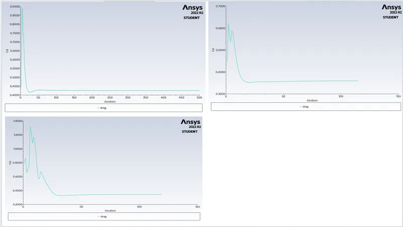
- The drag coefficient plot for a refined case. (For velocity of 25m/sec, the drag coefficient should be around 0.33).
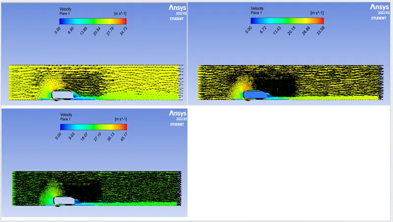
- The vector plot clearly showing the wake region.
- Perform the grid independency test and provide the values of drag and lift with each case.
Ahmed body:
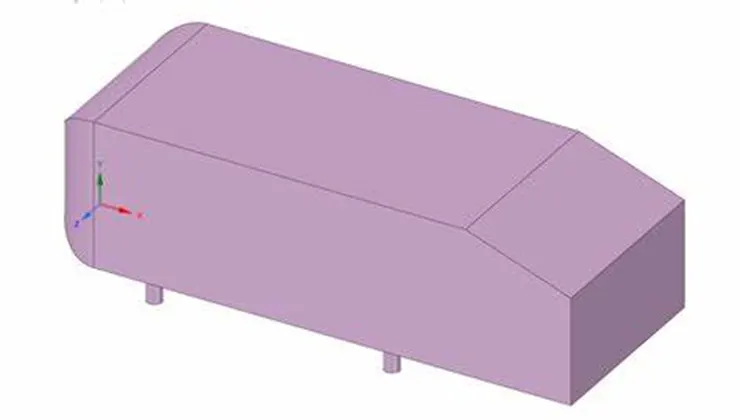
Ahmed body is a simplified car model geometry. Ahmed body is used to capture the basic flow characteristics of an automobile. CFD is used to study the aerodynamic behaviour of Ahmed body.
The Ahmed body is a benchmark model widely used in the automotive industry for validating simulation tools. The Ahmed body shape is simple enough to model, while maintaining car-like geometry features.
Ahmed body was developed by S.R. Ahmed & presented in his research paper “Some Salient Features of the Time-Averaged Ground Vehicle Wake” in 1984. This body is used as a generic car body because it captures all the essential flow features around an automobile and is easy to model.
The simple model makes meshing easier, reduces the computational power required and the time taken to run the simulations. Hence the body is widely used by researchers & engineers to validate their numerical model or CFD codes and sometimes without even wind tunnel testing as vast experimental data is already available (for different scale models of Ahmed body) from validation studies over the years.
Negative pressure in the wake region:
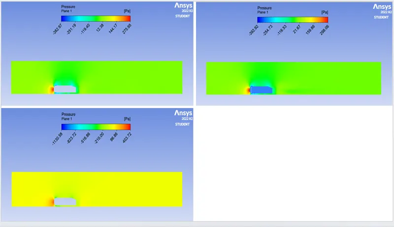
- Negative pressure in the wake region the fluid as it flows Ahmed body there would be stagnation of air particles at the front of the Ahmed body and pressure would be more which can be seen from the pressure contour, then there would be gradual increase in the acceleration of the air particles till the start of the slant angle
- Reason for negative pressure in the wake region: The path lines showing the exact circular motion or vorticity generation just at the rear end of the car. The separation takes two regions of distribution. One at the upper part of the rear and the other at the lower part of the rear end.
- The flow around the vehicle is characterized by high turbulent and three-dimensional flow separations as well as there is a growing need for more insight into the physical features of these dynamical flows. The Ahmed Body is a simplified car, used in the automotive field to investigate the flow analysis and find the wake flow around the body.
Point of separation:
The rear slant angle of the Ahmed body has a considerable effect on the flow separation at the rear end and the 25-degree configuration, particularly, is the one of the critical cases where flow experiences both flow separation and reattachment over the rear slant surface.
The flow separation happens at different points for a body based on the type of flow, basically, Laminar or Turbulent. For the laminar flow, the flow separation happens quickly resulting in minimal shear drag and a large pressure drag which forms a wake region (low pressure) behind the body, while for the turbulent flow, the flow separation is delayed causing minimal pressure drag but a slight increase in shear drag since the velocity profile is thicker for turbulent flow in comparison with laminar flow.
Challenge approach:
In this challenge we have to use ANSYS Fluent solver to create the geometry and perform unstructured tetra CFD mesh. We have to use five major steps in this challenge, there are Geometry, mesh, set-up, solution, result. We have to follow these steps. So, in this challenge we have to create
Case Element Outer Enclosure Inner enclosure Car wall
size in (mm)
Case 1 250 100 5
Case 2 100 50 3
Case 3 80 45 3
with boundary definitions, setup the physics of fluid flow and run the iterations to get solutions, using post processing to interpret the data in form of plots, contours, vectors, streamlines etc., With velocity of 25 m/s and k-epsilon model we shall study grid independence for Ahmed Body with RANS. When we say grid independence study, we shall study for 3 cases as follows.
Step 1: Geometry
First, we have to upload the given model (Ahmed body) in ANSYS fluent software.
Next step is we have to do create two enclosers for given Ahmed body.
In the space claim tap first we have to click prepare option and then we have to click enclosure option we have to create two enclosures for this Ahmed body, below I mentioned the measurements of the enclosures so we have to follow this.
Front (m) Back (m) Top (m) Bottom (m) Side (m)
Outer enclosure 2 5 1 0 0.5
Inner enclosure 0.5 1 0.5 0 0.25
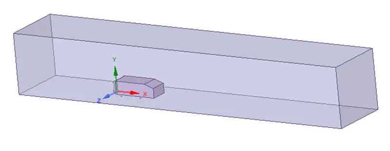
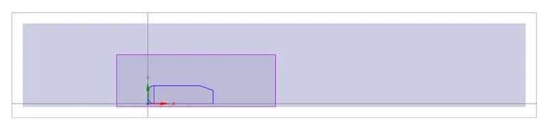
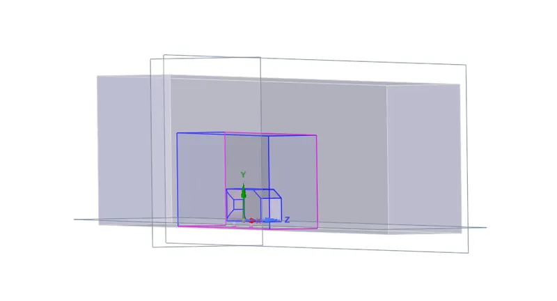
Once we created the enclosures after that we have to go design option and then we have to create the planes for x, y and z plane. And then we have to split the Ahmed body by using split body option. There are two enclosures, so we need to perform some more operations so that they behave as a single flow domain during study. INTERFERENCE option automatically identifies interference in objects and rectifies them, SHARE TOPOLOGY option shares the faces between 2 fluid volumes in this case the interface of outer and inner enclosures. And finally, we completed geometry the ANSYS fluent workbench is indicate the green tick symbol we have to move next process of meshing.
Step 2: Meshing
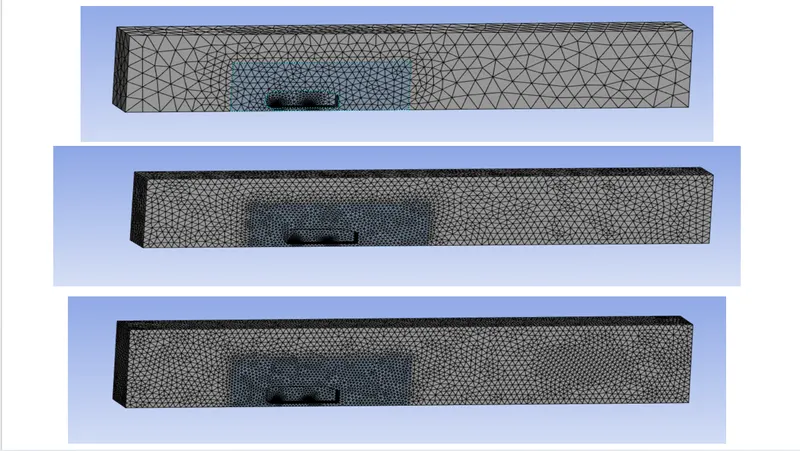
Next process is Meshing so we have clicking on the GENERATE MESH should create a mesh automatically. And selecting the inner enclosure by BODY select option and in MESH > INSERT > SIZING we should be able to select and input desired mesh sizes for car wall and inner enclosure. For outer enclosure, we can input size at the mesh details itself. We shall use INFLATION layers for the car wall with 0.5 as first layer thickness with 6 layers and 1.2 as growth factor. Since we already used share topology option, the mesh should look good. And then we should give the named selection option to create the inlet, outlet, symmetry and car wall. We have to follow the three cases the same procedure to generate mesh. Below I mentioned the three cases meshing element size we have to follow this element size for three cases.
Case Element Outer Enclosure Inner enclosure Car wall
size in (mm)
Case 1 250 100 5
Case 2 100 50 3
Case 3 80 45 3
Once we completed the meshing process for three cases after that we have to move next set-up process.
Step 3: Set-up
In this challenge the third step is set-up process and right click and give start. we shall select Type: Pressure based, Velocity Formulation: Absolute, Time: Steady. Under the Physics tab, we can turn on viscous and select k-epsilon > Enhanced wall treatment as well. Under the materials we shall select air as our default material with material type as fluid.
The cell zone conditions, select the volume and it should show type as fluid by default. We can proceed to define boundary conditions, as follows
Inlet X: velocity magnitude = 25 m/s Outlet should be a pressure outlet.
For generating surface reports, click on the Solution > Reports > Definitions > New > Force Report > Drag coefficient for the drag coefficient over the cylinder wall.
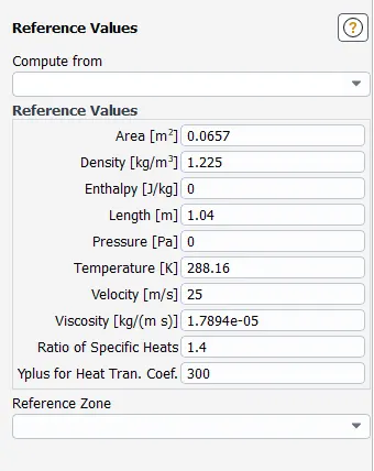
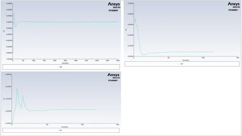
Similarly, we can make a report for lift coefficient. We shall input compute from INLET in reference values and in the initialization as well. Now, it's time to start the simulation. In order to start the simulation for the above set up physics, we need to initialize the entire flow field by clicking on the t=0 initialize icon.
In the Run Calculation we can input the number of iterations to be run (in this case 500) and clicking on the Calculate should start the iterations.
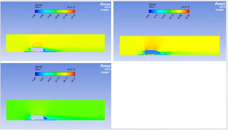
We need velocity and pressure contours as well, to get them we can create a transverse cut plane XY plane and make new contour in Results > Graphics > Contours > New pressure for pressure contour and velocity for velocity contour. Ansys Fluent Simulation Report which is automatically generated with all the information of the simulation in it. This can be exported as a PDF also. Once we completed the set-up process after that we can able to move solution step. Beow the image is represent the reference values for the set-up process.
Reference values:
Step 4: Solution
Some solutions are completed in the set-up process itself . So we have to move result process.
Step 5: Result
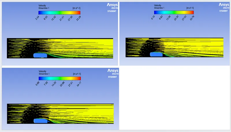
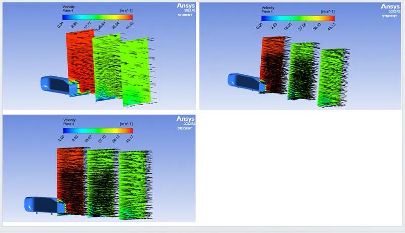
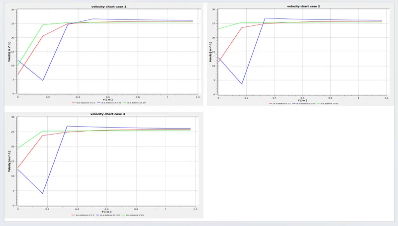
Finally, we have to right click and open the Result option should open the Post processor. In the result tab we have to see the default view is a wireframe model, we can create a plane in XY to view contours and vectors. Selecting the Vector and selecting the plane creates a velocity vector. We have cretae the streamline contours three cases for velocity vector by using streamline option. And then we shall create the lines at distance of 1.05 m, 1.5 m, 2 m away from the tail of the car to study the velocity chart on the same. Plots can be created using the CHART option. For Case 1, 2and Case 3, we shall repeat the same except for changing the grid size in meshing step. We can simply DUPLICATE case 2 fluent file and edit in it.
Below I attached the results of velocity, pressure contours, plots and streamline contours velocity charts and vector plots for three cases.
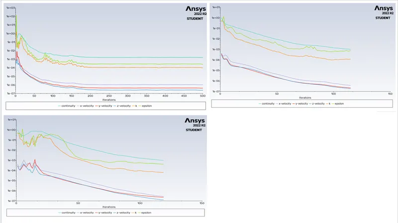
Case 1, 2 and 3 Residual plots:
Case 1, 2 and 3 Drag plots:
Case 1, 2 and 3 Lift plots:
Case 1, 2 and 3 Velocity contours:
Case 1, 2 and 3 Pressure contours:
Case 1, 2 and 3 velocity vector contours:
Case 1, 2 and 3 velocity streamline contours:
Case 1, 2 and 3 vertical plane at the distance of 1.05m, 1.5m and 2mvelocity vector contours:
Case 1, 2 and 3 vertical plane velocity charts:
Conclusion:
Finally, we conclude from the results of all 3 cases, and we got the drag coefficient and lift coefficient values.
Case 1 Case 2 Case 3
Outer enclosure 250 100 80
Inner enclosure 100 50 45
Car wall 5 3 3
Drag coefficient 0.425 0.359 0.334
Lift coefficient 0.203 0.240 0.223
Inferences:
From this challenge the expected drag coefficient of 0.33 at the case 3. As the drag coefficient decreases the lift coefficient increases. Where the case 2 and 3 in finer mesh the iterations are converged around 120 iterations itself. So, mesh size impacts the convergence as well. The distance from the tail of car Vs Velocity plot shows that as the distance from tail increases the velocity is more.
References:
https://flowvision.ru/images/articles/2020/Add_files/Ahmed_1984.pdf