Week 3 - External flow simulation over an Ahmed body.

OBJECTIVE:

The objective of this project is to do an external flow simulation over Ahmed body and to study the nature of the flow in the wake region and forces such as drag and lift coefficient.

ABSTRACT:

AHMED BODY:

The Ahmed body is a geometric entity that represents a standard passenger car. The geometry was first proposed by Ahmed and Ramm in 1984 and was extensively used to study the effects of the geometry on the wake region. Over the years, numerous studies have been conducted on the Ahmed body both computationally and experimentally using wind tunnels.

The “Ahmed” body, has the form of a highly simplified car, consisting of a blunt nose with rounded edges fixed onto a box-like middle section and a rear end that has an upper slanted surface (like a “hatch-back” car), the angle of which can be varied. The model is supported on circular-sectioned legs or stilts, rather than wheels. Despite neglecting a number of features of a real car (rotating wheels, rough underside, surface projections, etc.) the Ahmed body generates the essential features of flow around a car, namely: flow impingement and displacement around the nose, relatively uniform flow around the middle and flow separation and wake generation at the rear.

Besides the analyses of the velocity field, the Ahmed Body is also used for drag force and lift force analyses and rolling, pitching and yawing moments. The slant angle on the back allows studying the separation region and its influence on the velocity profile and forces.

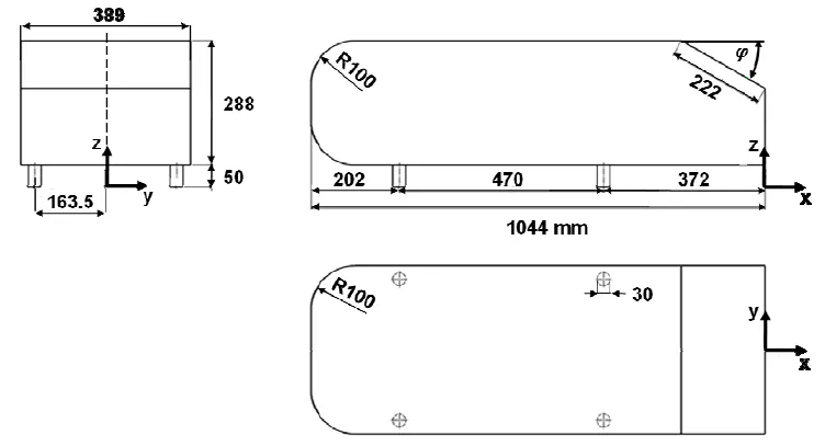
The geometry of the Ahmed body is shown in the figure below. The slant angle is adjustable and is the main variable model parameters in the experimental investigations. The Ahmed body, of length (L) 1044 mm, height (H) 288 mm, and width (W) 389 mm, was placed at 50 mm from the ground (G). The rear part of Ahmed body called as slant angle which influences drag and lift with its critical slant angle which is around 0-30 degree.

Ahmed Body:

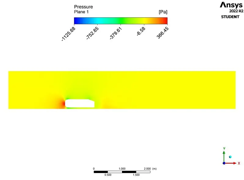
Negative pressure in the wake region

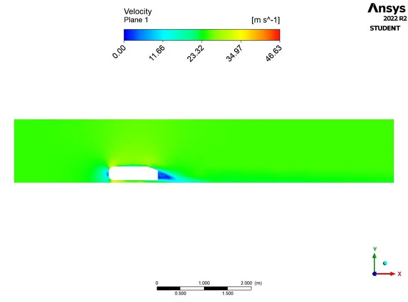
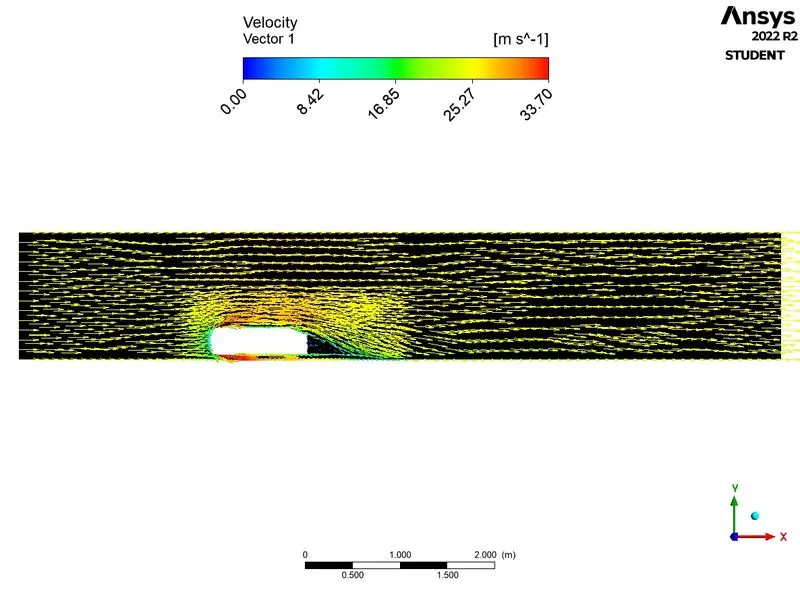
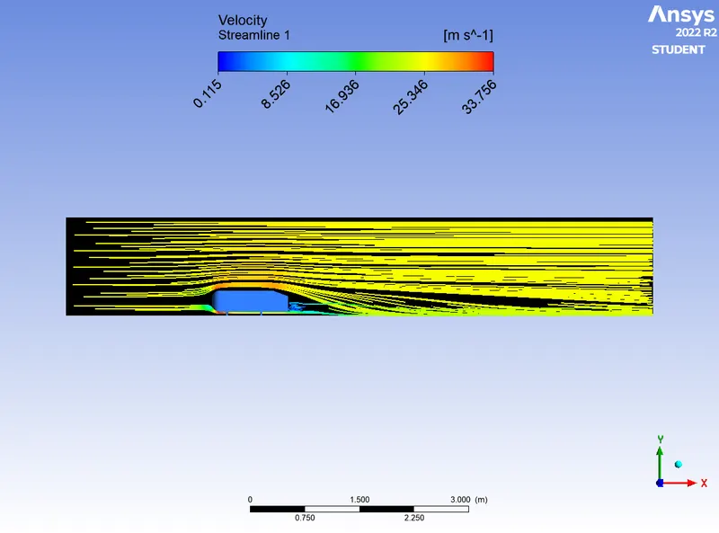
When the air moving over the vehicle it is separated at the rear end, it leaves a large low-pressure turbulent region behind the vehicle which is known as the wake. This contributes to the formation of pressure drag which affects the vehicle performance.

When the vehicle is moving at a certain velocity the fluid imparts viscous force to the vehicle as long as it is in the viscous sublayer of the boundary. When the fluid reaches the rear end of the vehicle it gets detached from the surface of the body causing negative pressure in the wake region. The movement of the fluid around the vehicles depends on the geometry of the car and the Reynolds number.

Modelling Procedure:

1: Pre-Processing.

• Open Ansys Workbench→under Analysis system select Fluid flow(fluent) drag and drop it in Project schematic → Geometry → New spaceclaim geometry.
• File select the appropriate file and then Open the file.
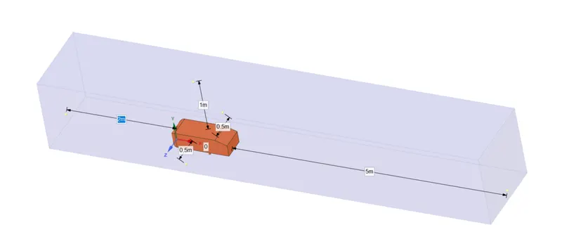
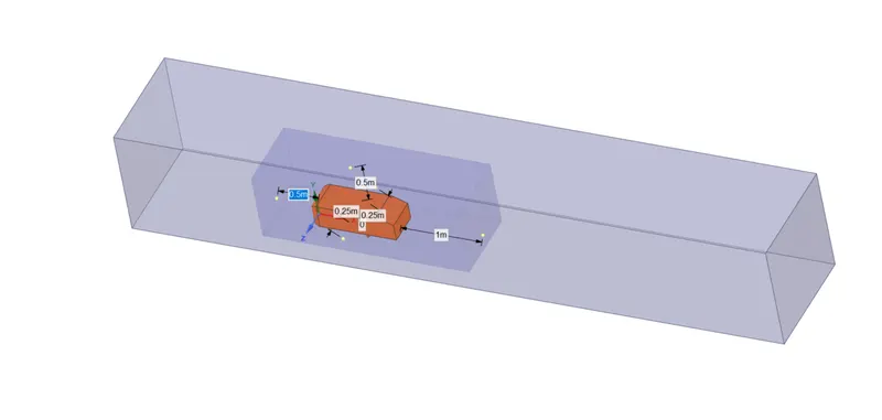
• The given problem is external aerodynamic simulation. A wind tunnel is created over the Ahmed body using the Enclosure option in Spaceclaim. This outer enclosure contains a smaller, inner enclosure (for local refinement) which in turn contains the surface of the Ahmed body.
• Since we created two enclosures, they will interfere with each other, to clear the interference there is option called Interference in spaceclaim. This interference option will automatically detect if there are any interference present and then it will clear it.
• In order to have common node points between the enclosures we are using Share topology option to share the node points.
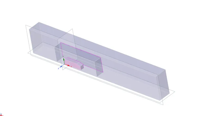
• The Ahmed body is a perfectly symmetric body we can run the simulation by considering the only half body. We can use Split body command to split the body. This helps to save a lot of computational cells that can be used to further refine the wake region.

Outer Enclosure:

Inner Enclosure:

Split Body:

2: Meshing.

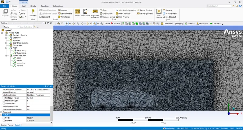
• We will proceed with mesh generation for required mesh element length using the Sizing and Inflation options. Mesh `rarr` Details of “Mesh” `rarr` Element Size then specify the required mesh length. For Inflation Inflation `rarr` Geometry select the geometry and define the inflation layer thickness and no of inflation layers.
• Then we should appropriate names for parts of the geometry to make it easier while working on simulation.
• Using the y+ concept, we calculated first layer thickness as 0.4mm.

3: Simulation.

• Setting up for Physics. Choose pressure-based solver and steady state condition.
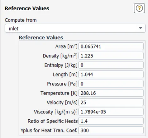
• Define the conditions under Reference values such as area and length. Area=0.065741 m^2 and Length=1.044 m.
• The turbulence model we are using is K-epsilon turbulence model with Enhanced wall treatment.
• Then define the inlet boundary conditions which is 25m/s.
• Then create the required surface plots. Like Drag and Lift plots.
• Initialize and run the simulation.

Grid Dependency test:

We have to ensure that the solution does not depend on the number of elements in the model. So, we run few simulations with different number of mesh elements. This is called Grid dependency test, where we decide the minimum number of elements required to make sure the solution is acceptable.

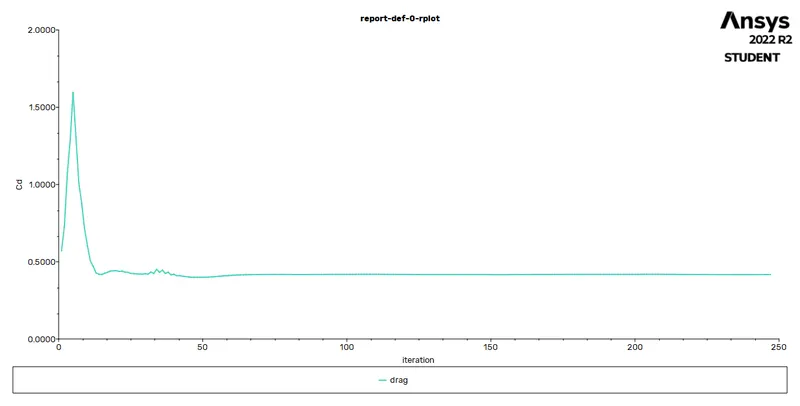
For the given geometry, we would run grid dependency test till we reach a point where we get solutions with acceptable error range (<0.5%). We will use the average value of drag coefficient as the parameter to obtain the ideal computational grid.

Case 1:

Outer Enclosure=250mm.

Inner enclosure =100mm.

Legs=5mm.

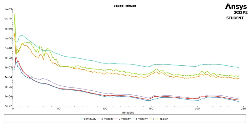
Residual Plot:

Drag Coefficient:

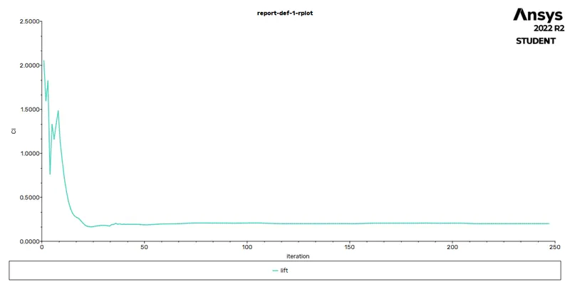
Lift Coefficient:

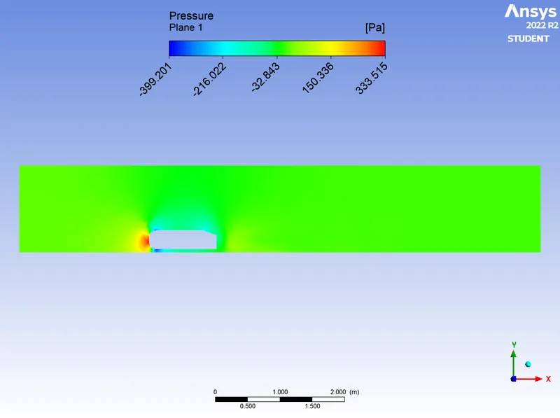
Pressure contour:

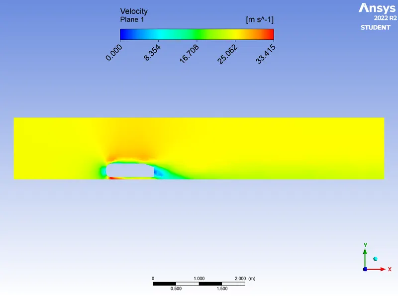
Velocity Contour:

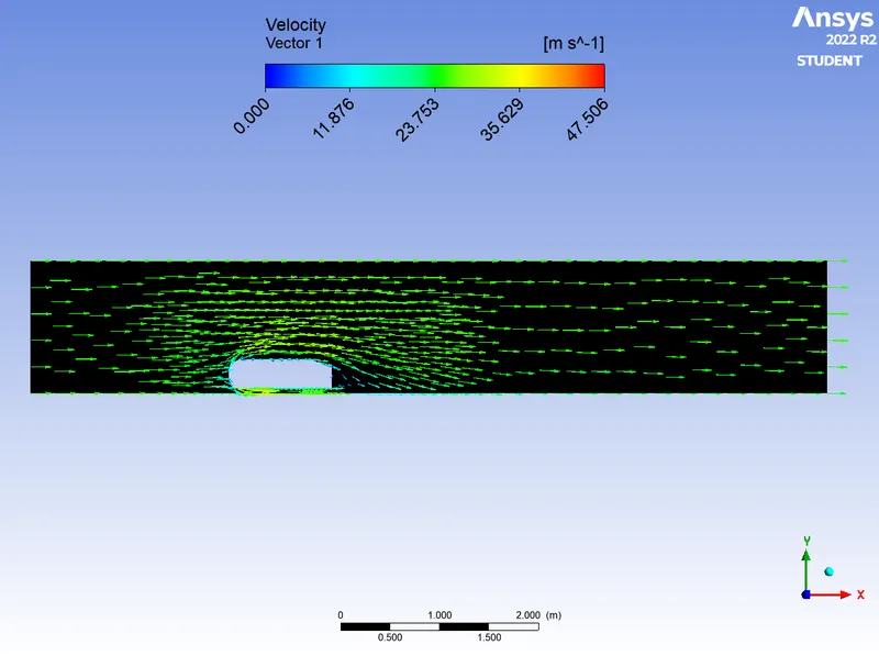
Velocity Vector:

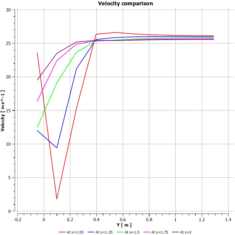
Velocity Comparison:

Case 2:

Outer Enclosure=100mm.

Inner enclosure =50mm.

Legs=3mm.

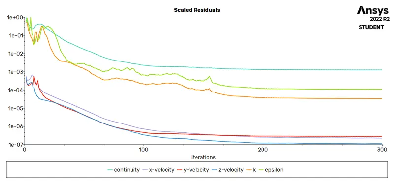
Residual Plot:

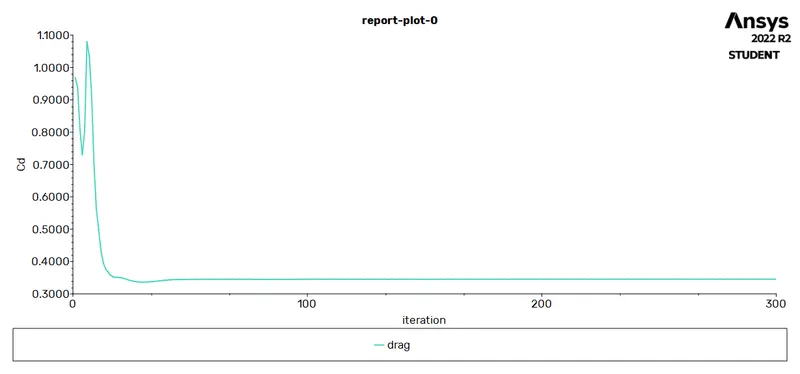
Drag Coefficient:

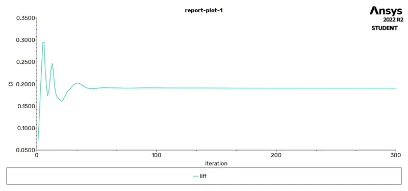
Lift Coefficient:

Pressure contour:

Velocity Contour:

Velocity Vector:

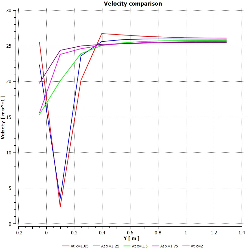
Velocity Comparison:

Case 3:

Outer Enclosure=85mm.

Inner enclosure =35mm.

Legs=1mm.

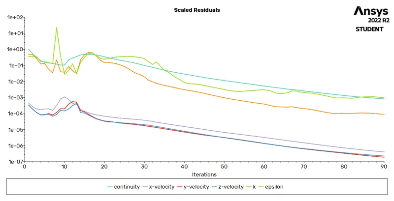
Residual Plot:

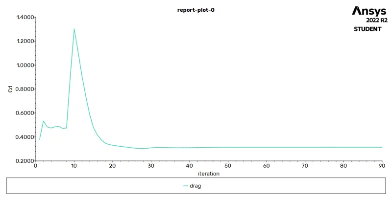
Drag Coefficient:

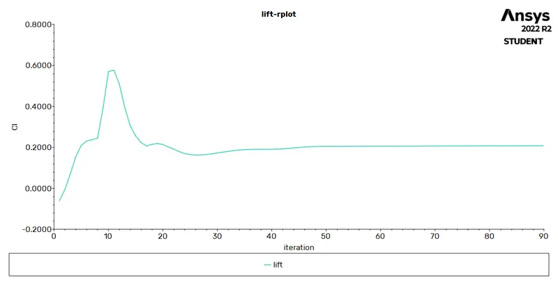
Lift Coefficient:

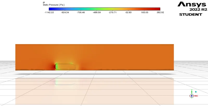
Pressure contour:

Velocity Contour:

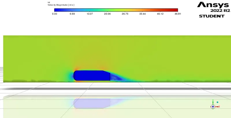
Velocity Vector:

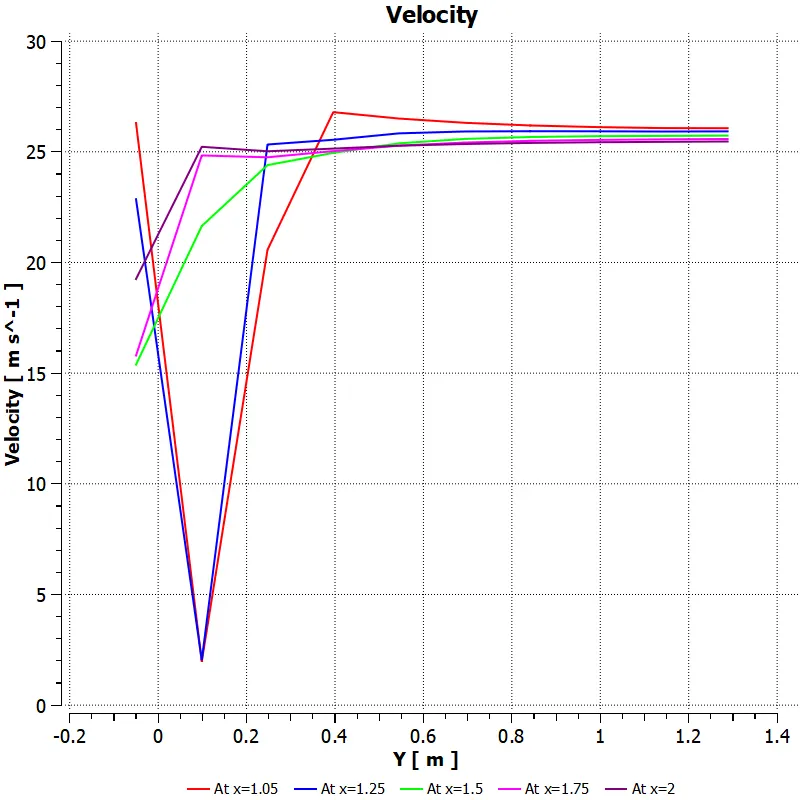
Velocity Comparison:

Mesh parameter (mm)	No. of elements	Drag coefficient	Lift Coefficient
250 x 100 x 5	57654	0.4171	0.2008
100 x 50 x 3	135032	0.3449	0.1905
85 x 35 x 1	301752	0.3142	0.2078

From the data, we can decide that the mesh more no of elements is ideal for this simulation.

CONCLUSION:

The flow over the Ahmed body is conducted and the wake region is visualized using Vector and Contour plots and analyzed. The coefficient of drag and coefficient of lift is estimated. The point of separation and its influence is talked upon. The grid Independence test is conducted.