Week 3 - External flow simulation over an Ahmed body.

Aim: To study the turbulence and the nature of the flow in the wake region of Ahmed body.

Introduction:

Experiments performed to study the physics of certain phenomenon is costly and time-consuming. Numerical simulation is developed and used to reduce the time needed to study the nature and physics of the system of interest. This method indeed provides results very fast compared to experiments but they lack a bit in terms of accuracy. If the experiments take a month to produce results, simulation might take a day and give us results 90% accurate. In the fast-paced world, where developing various solutions require faster results, engineers make a delicate balance between the accuracy and time taken as necessary.

All fluid flows are governed by three equations -Continuity, momentum and energy equations. We need to solve these equations for the given conditions to understand the fluid behavior. Computers are incapable of solving these equations in their integral and differential forms. So, we can divide our geometry into many tiny elements (called mesh) and modify the governing equations into difference equations that can be solved by the computer. We apply these difference equations for all the elements in the geometry and generate an approximate solution. It is hence necessary to validate these results against the experimental data.

The number of difference equations, for a given problem varies with the nature of physics involved. We typically solve a finite number of equations at all the elements. These equations are grouped together, called a turbulence model. A lot of work has been put into developing and improving the turbulence models and the work still goes on today. Examples of turbulence models are S-A, k-epsilon, k-omega etc.

Theory:

Ahmed body is a simplified version of the car body. This model has all the parts of a car that would affect the physics of the air flow significantly. Since this is a simple design, it is also used to validate the turbulence models against the experimental data.

The rear part of Ahmed body called as slant angle which influences drag and lift with its critical slant angle which is around 0-30 degree.

Y+ concept:

This is the concept that enables us to calculate the size of the mesh element which can capture te effects of boundary layer for the given body and input parameters.

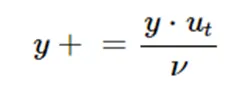
Where y+ = thickness of the first mesh element,

Y = distance from the wall.

U_t = frictional velocity,

nu= dynamic viscosity.

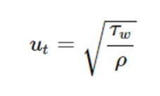
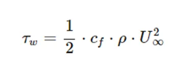
Where = wall shear stress.

C_{f =} skin friction coefficient.

Drag-coefficient:

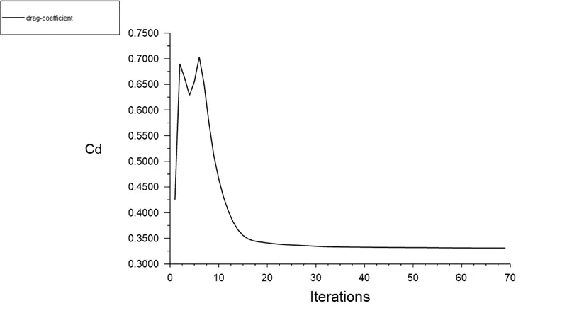
When the fluid flows over the stationary body or vice-versa; the body offers a resistance to the fluid flow. This causes the fluid to exert force on the body which is termed drag-force. A non-dimensional parameter used to study this nature is called drag-coefficient (C_d).

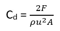
Where F = drag force (N)

ρ = density of the fluid (kg/m³)

u = flow velocity (m/s)

A = hydrodynamic area (m²)

Lift-coefficient:

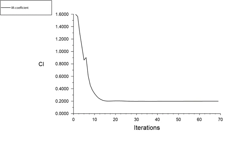
When the fluid stream is split into two parts by the body, the pressure difference between the two streams causes a force to act through the body termed as Lift force. A non-dimensional parameter used to study this nature is called lift-coefficient (C_L).

Where F = Lift force (N)

ρ = density of the fluid (kg/m³)

u = flow velocity (m/s)

A = hydrodynamic area (m²)

Modelling Approach:

The work flow in Ansys Fluent would follow four steps:

1. Geometry creation.
2. Mesh generation.
3. Pre-processing settings and simulation.
4. Extracting results.

Geometry creation:

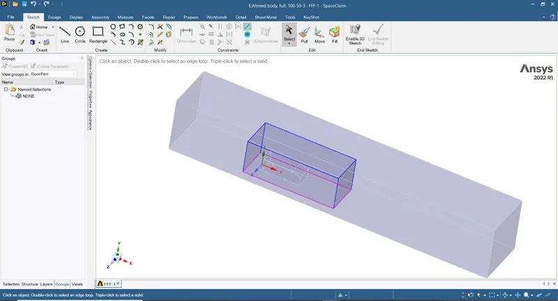
We drag and drop the Fluent module to create the standalone system. We open the geometry editing section- Space claim and import the given model and create a rectangular computational domain.

We create another small domain to improve the mesh near the body. We use Interference command for proper flow simulation across the two domains. We split the model into two appropriate halves using Split command.

Mesh generation:

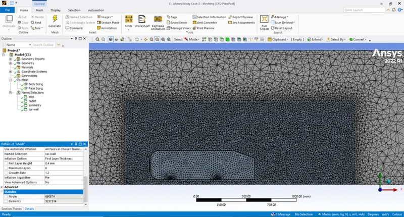
We will proceed with mesh generation for required mesh element length using the Sizing and Inflation options. We use Mesh -> Insert -> Sizing, to specify the number of the mesh elements in the given edge. We use Mesh -> Insert -> Inflation, to create inflation layers near the car boy.

We assign appropriate named selections to make it easier to work in the simulation section later. Here, we assigned the flow inlets, outlet, wall and symmetry. We close the window and the changes are updated in the system.

Using the y+ concept, we calculated first layer thickness as 0.4mm.

Pre-processing settings and Simulation:

We would proceed to Setup the conditions of the model. The process flow would be as follows:

1. Check the mesh in the solver.
2. Choose the turbulence model.
3. Specify boundary conditions.
4. Create necessary surface plots that we need to investigate.
5. We initialize and run the simulation for given number of iterations.
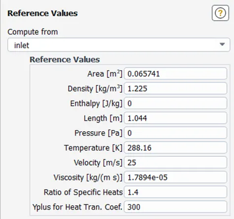
6. We set the reference values for area and length as 0.065741m² and 1.044m.

Extracting results:

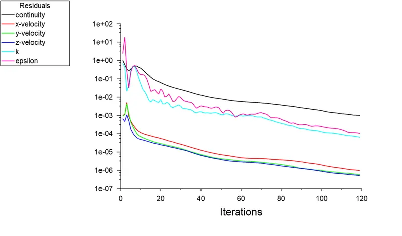
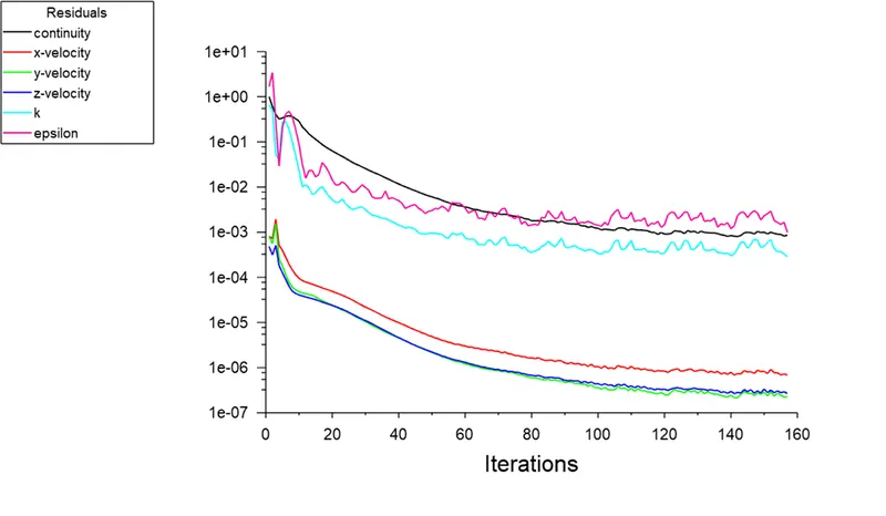
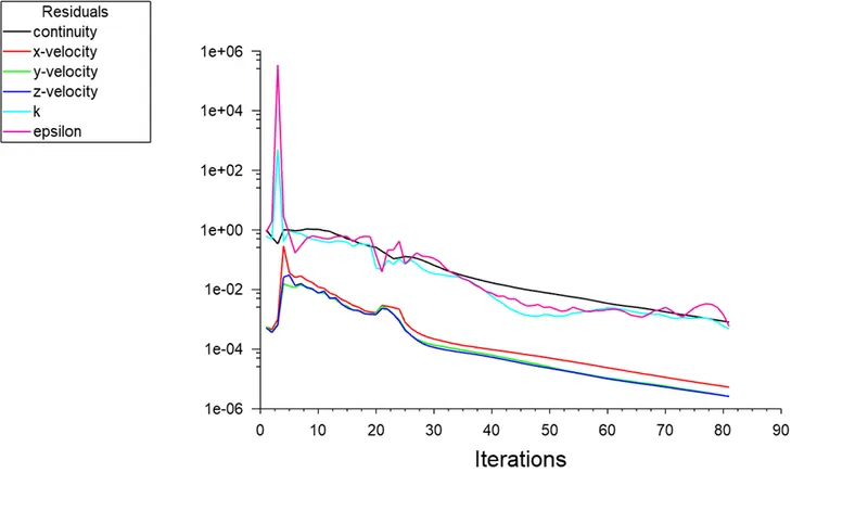
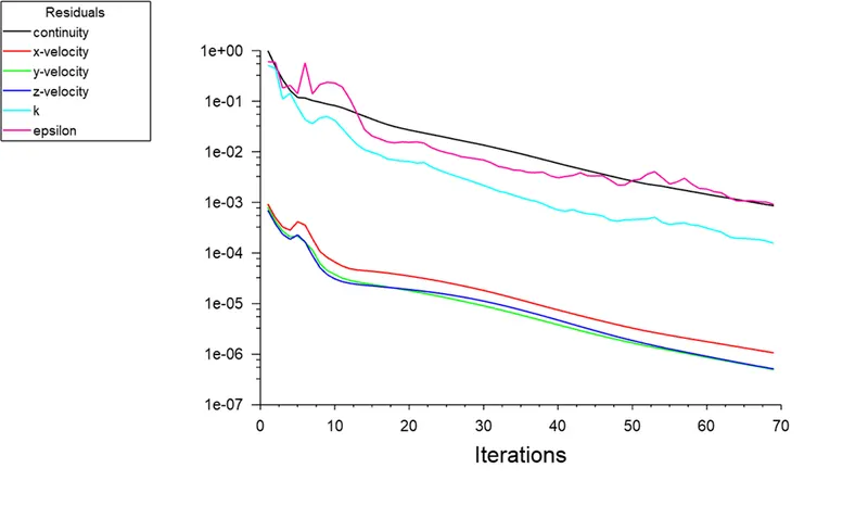
We open the results section where we can use various visualizing tools like transparency and colouring the created surfaces with the instantaneous variables like temperature, velocity and obtain contours, charts and plots. We need to run the simulation until the residual values are either reach the convergence criteria or display a periodic pattern.

Settings used for current simulation:

We used Pressure-based solver, absolute velocity formulation, steady state simulation.

We used standard k-epsilon turbulence model with enhanced wall treatment. We use air as the working media.

We would use fluid velocity as 25 m/s and update the reference values as follows:

Grid Dependency test:

We have to ensure that the solution does not depend on the number of elements in the model. So, we run few simulations with different number of mesh elements. This is called Grid dependency test, where we decide the minimum number of elements required to make sure the solution is acceptable.

For the given geometry, we would run grid dependency test till we reach a point where we get solutions with acceptable error range (<0.5%). We will use the average value of drag coefficient as the parameter to obtain the ideal computational grid.

For this study, we would use the grid inputs as the following function:

Element size in outer domain x size in inner domain x size in the legs of the body.

Case 1- 250mm x 100mm x 5mm:

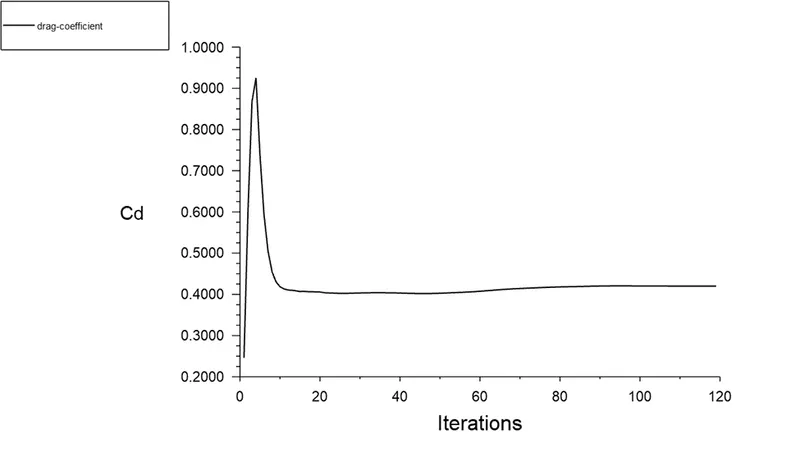
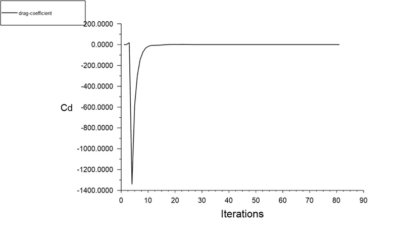
Drag coefficient:

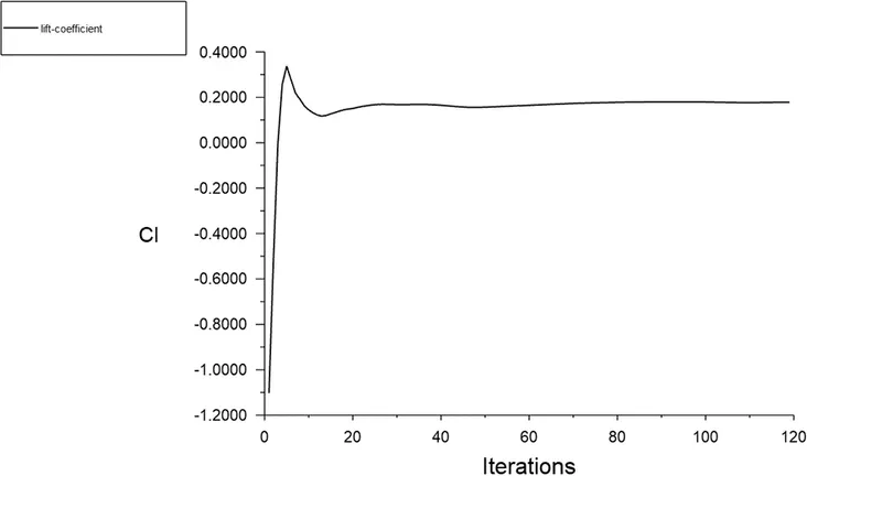
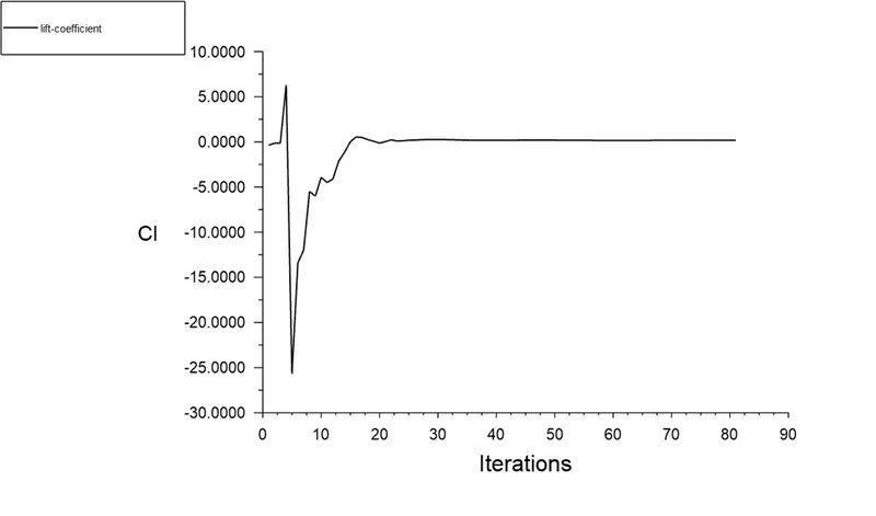
Lift coefficient:

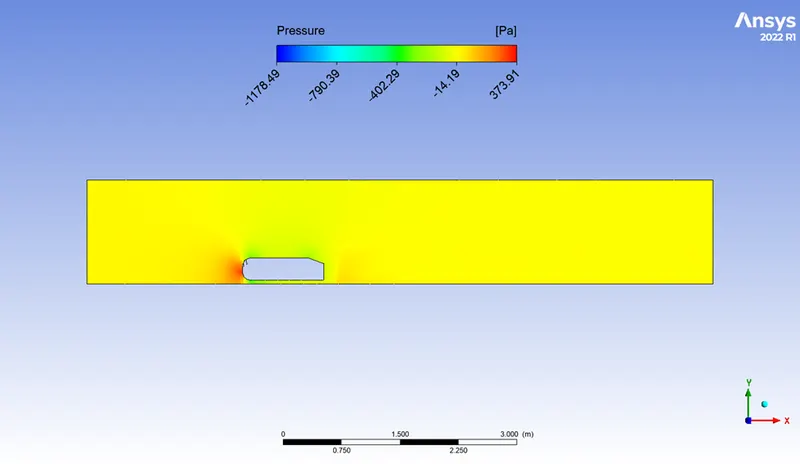
Pressure contour:

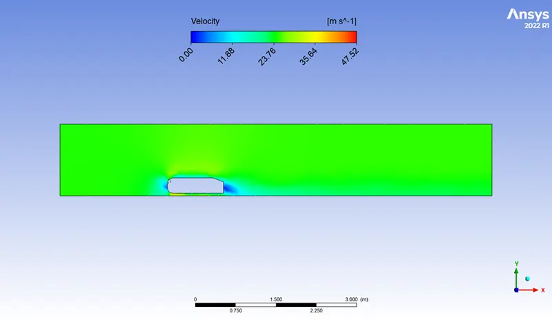
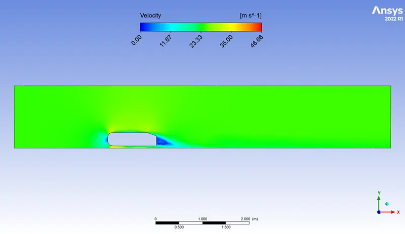
Velocity contour:

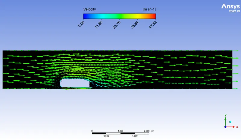
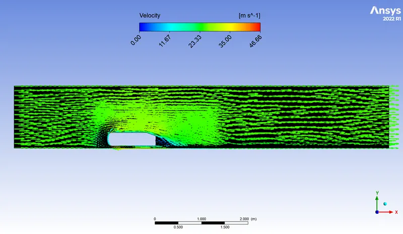
Velocity vector:

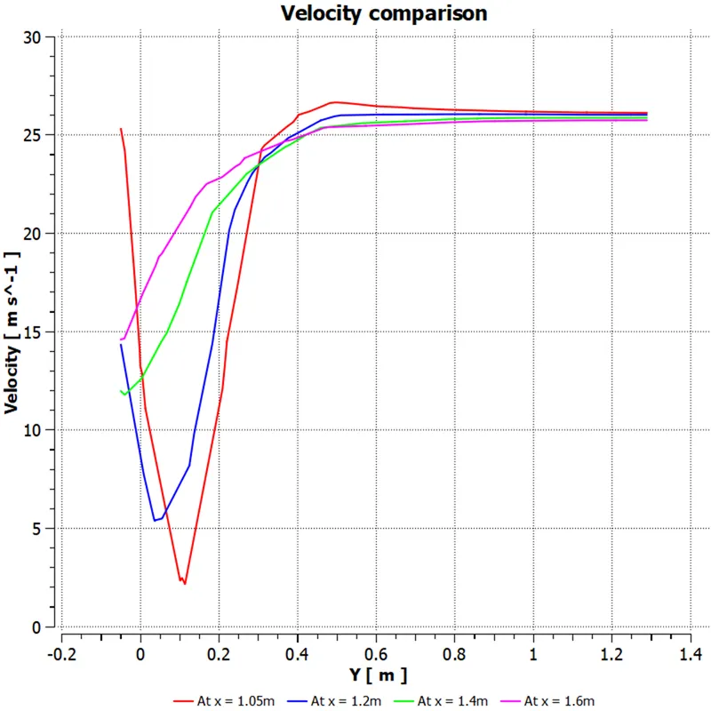
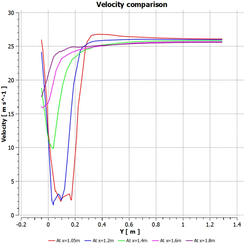
Velocity comparison at various x-coordinates:

The average drag coefficient value obtained for this simulation is 0.4201.

Case 2- 200mm x 80mm x 4mm:

Scaled residuals:

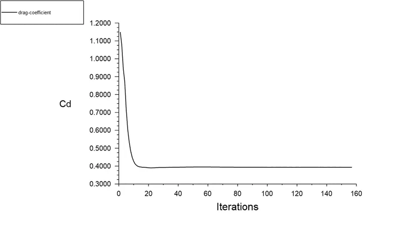
Drag coefficient:

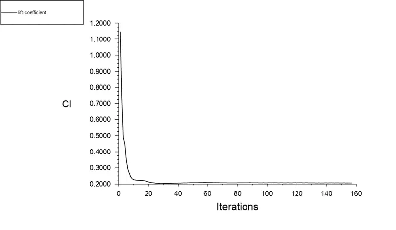
Lift coefficient:

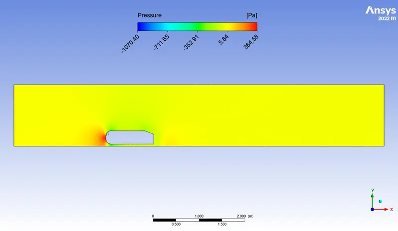
Pressure contour:

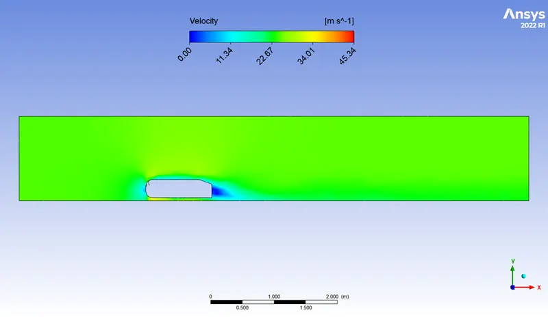
Velocity contour:

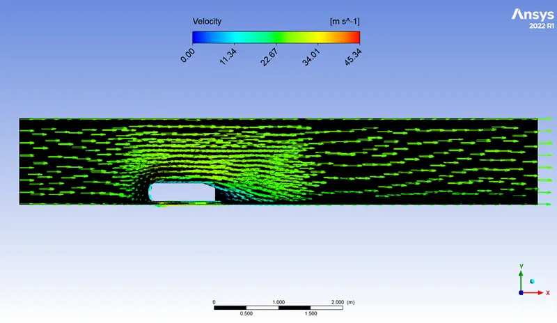
Velocity vector:

Velocity comparison at various x-coordinates:

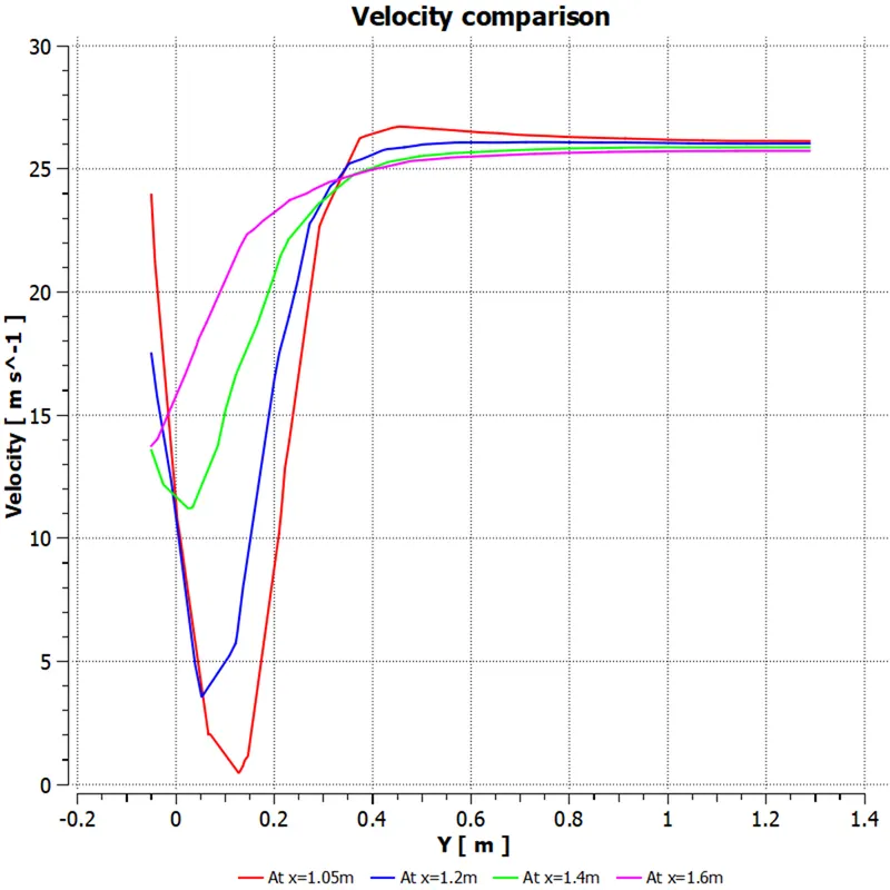
The average drag coefficient value obtained for this simulation is 0.3933.

Case 3- 150mm x 70mm x 4mm:

Scaled residuals:

Drag coefficient:

Lift coefficient:

Pressure contour:

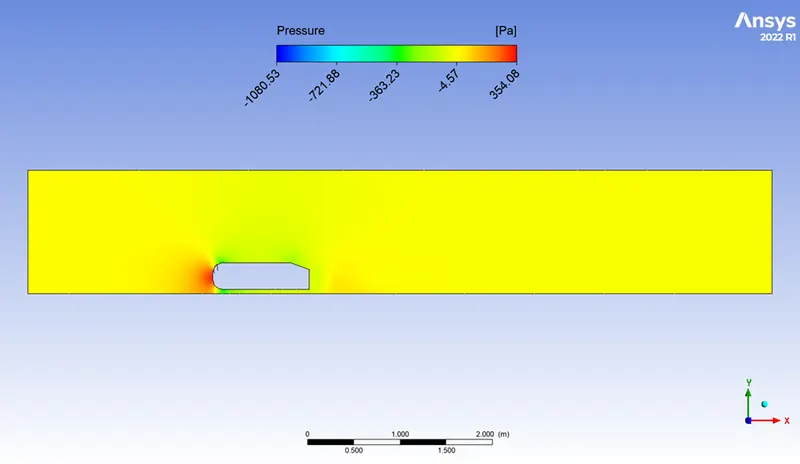
Velocity contour:

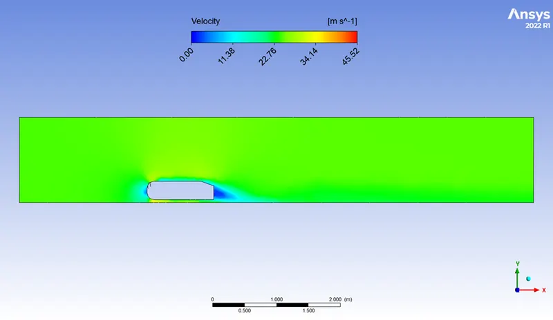
Velocity vector:

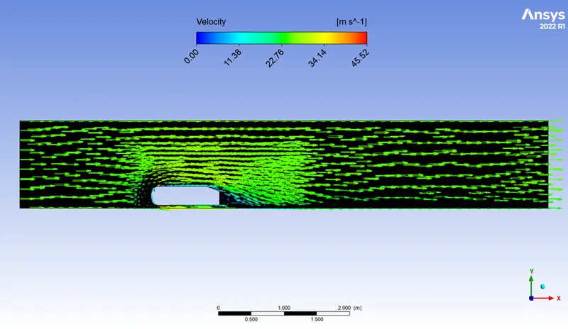
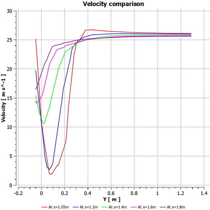
Velocity comparison at various x-coordinates:

The average drag coefficient value obtained for this simulation is 0.3907.

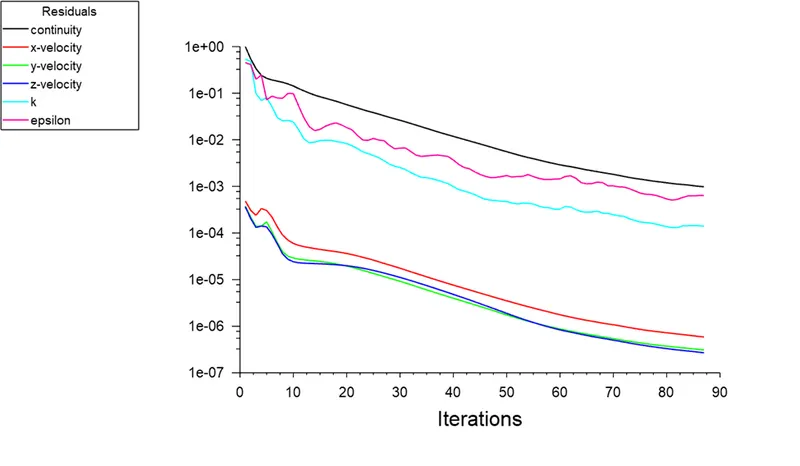
Case 4- 100mm x 50mm x 3mm:

Scaled residuals:

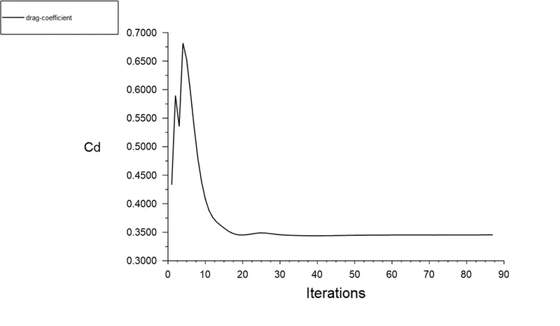
Drag coefficient:

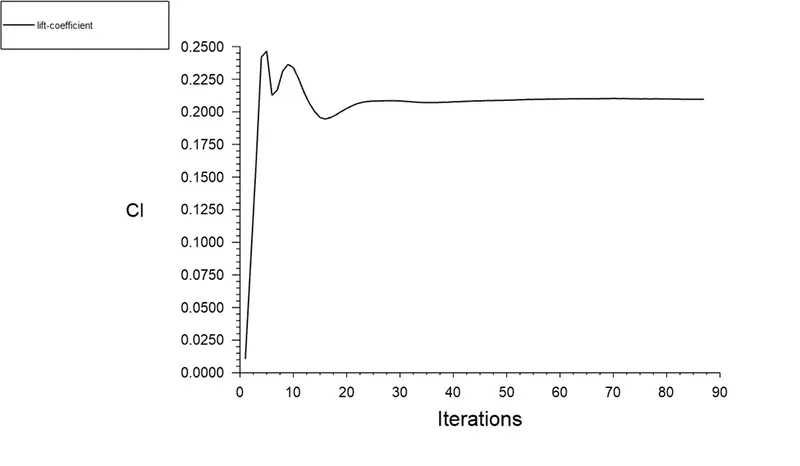
Lift coefficient:

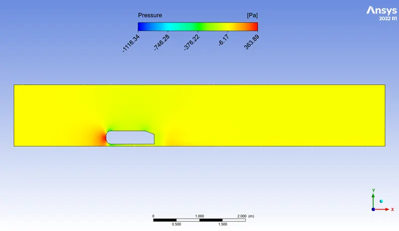
Pressure contour:

Velocity contour:

Velocity vector:

Velocity comparison at various x-coordinates:

The average drag coefficient value obtained for this simulation is 0.3454.

Case 5- 80mm x 45mm x 3mm:

Scaled residuals:

Drag coefficient:

Lift coefficient:

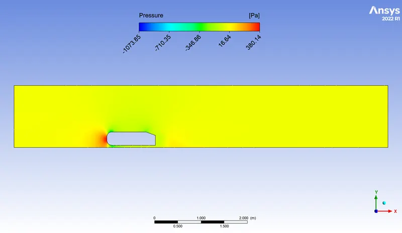
Pressure contour:

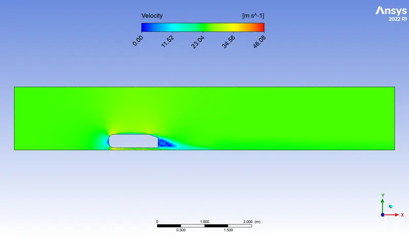
Velocity contour:

Velocity vector:

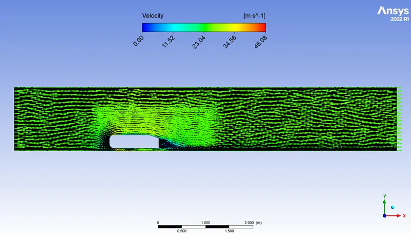
Velocity comparison at various x-coordinates:

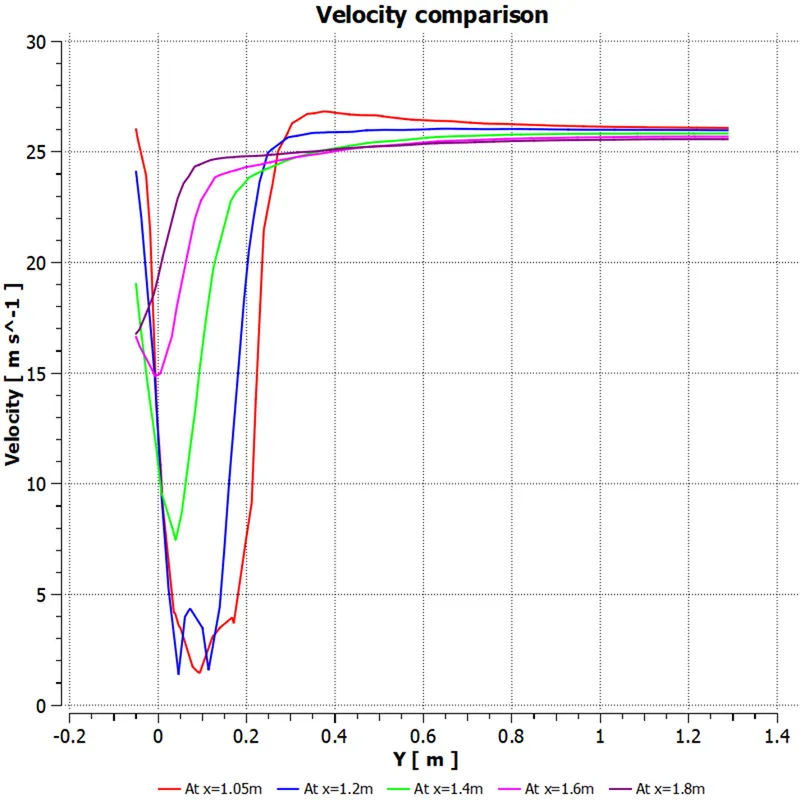
The average drag coefficient value obtained for this simulation is 0.3309.

Case 6- 70mm x 40mm x 2mm:

Scaled residuals:

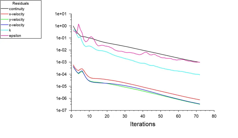
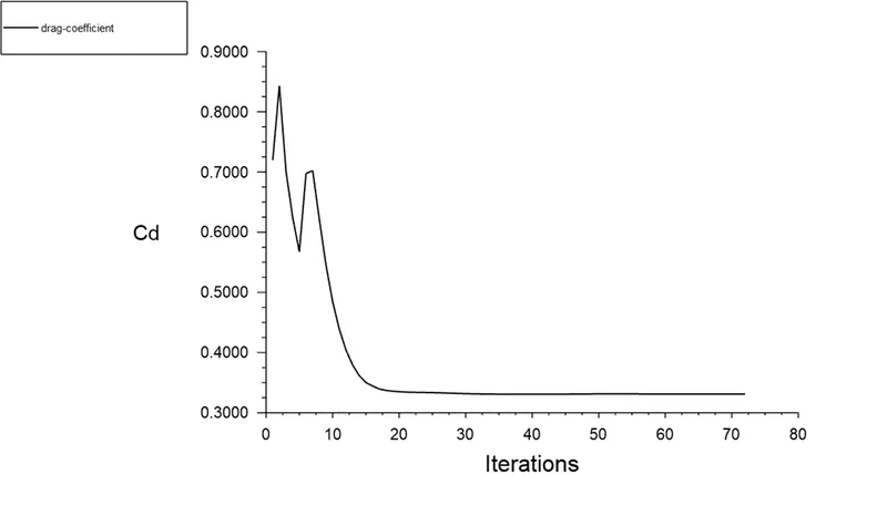
Drag coefficient:

Lift coefficient:

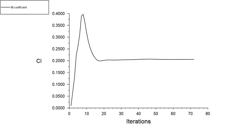
The average drag coefficient value obtained for this simulation is 0.3317.

The drag value obtained for the above mentioned six cases and the deviation of the parameter w.r.t. previous value is tabulated.

Mesh parameter (mm)	No. of elements	Drag coefficient	Error w.r.t. previous value (%)
250 x 100 x 5	58640	0.4201	-
200 x 80 x 4	83795	0.3933	6.45
150 x 70 x 4	100029	0.3907	0.66
100 x 50 x 3	205140	0.3454	11.59
80 x 45 x 3	259072	0.3309	4.2
70 x 40 x 2	382855	0.3317	0.24

From the above data, we have decided the mesh with parameters 80mm x 45mm x 3mm is ideal for the simulation. The post-processing images for other simulations are just presented for clear understanding of the dependence of the solution accuracy w.r.t. change in grid size.

Comparison between full and half body simulation:

Usually, for symmetric bodies; over the plane of symmetry, the body can be cut and we can get the result for the full body just by simulating the flow over the half body. This would reduce the number of mesh elements considerably and hence reduce computational effort. We can also verify the results obtained for both the cases.

Here we performed a full body simulation for 100mm x 50mm x 3mm grid and the drag coefficient values are found to be same.

Drag coefficient for half body:

Drag coefficient for full body:

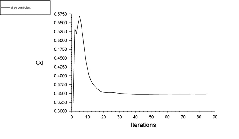
The number of mesh elements in full body analysis is 376118. Since the result is the same, we saved time and effort by using half body simulation.

Validation of results:

The drag coefficient value for the given body experimentally is 0.33. The simulated value for the finalized grid is 0.3309. The error is 0.27%. Hence the simulated result is validated.

Conclusion:

The errors in the experimental and simulated values are very small. Hence, we can say the turbulence model and the computational grid captured the flow physics accurately.

The velocity comparison graph gives us an insight into the wake region of the flow. It can be seen that from the rear end of the body the wake extended up to around 0.55m. The size of the wake region at a region is in proportion to the amount of drop in the velocity in the region. At 1.05m (rear end) velocity drop is the highest and it keeps reducing till 1.8m in the computational domain.

The blue-coloured region in all the velocity contours all have reversal of the velocity in the wake region. The slant angle in the rear part of the geometry has a sharp edge at which the flow separation occurs, the primary reason for wake to occur.

The lines are plotted at regular intervals in velocity comparison figures to allow us to find the extent of the wake region.

References:

1. Lienhart, Hermann, Stoots, C, Becker, S., Flow and Turbulence Structures in the Wake of a Simplified Car Model (Ahmed Model), Notes on Numerical Fluid Mechanics, Vol 77, 2002/01/01.
2. JOUR, Meile, Walter, Brenn, Günter, Reppenhagen, Aaron, Lechner, Bernhard, Fuchs, Anton, Experiments and numerical simulations on the aerodynamics of the Ahmed body, Vol 3, 2011/03/01.