Week 3 - External flow simulation over an Ahmed body.

Aim -->
To Analyse External flow simulation over an Ahmed body (basic car model) using Ansys Fluent. Our focus will be to talk about pressure distributions, velocity contours, wake region near the Ahmed body. We also need to use a specific near-wall treatment in the turbulence model and compute the aerodynamic drag/lift coefficients.

Ahmed Body

Front Part

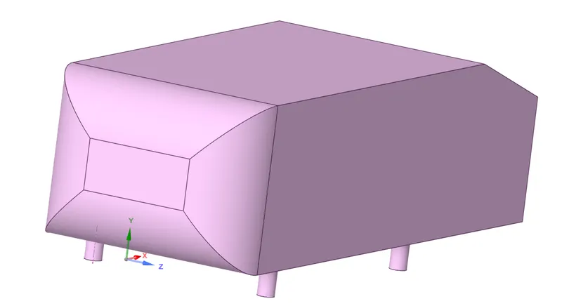
Rear Part

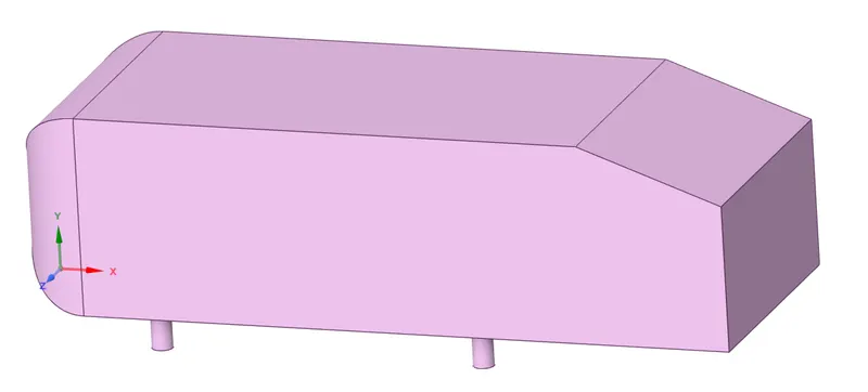
--> Ahmed body is a generic car model (simplified body). The airflow around the Ahmed body captures the essential flow features around a vehicle body and it also helps us to study the aerodynamics of the car model. Ahmed body is used to validate the numerical algorithm and turbulence model used in CFD codes. This is because the experimental data from wind tunnel testing is available for the Ahmed body. Once the numerical model is validated, it is used to design new models of the car. As we can see the model has curved features in the front part and a slant at the rear part, so it has geometric features of a car body.

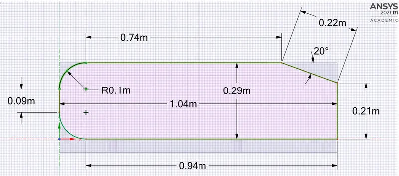
The Ahmed body was described originally by S. R. Ahmed in 1984. It has been heavily researched and a lot of experimental data (wind tunnel tests) are available. It was first published in the research paper “Some Salient Features of the Time-Averaged Ground Vehicle Wake” in 1984 by S. R. Ahmed. Since then, it has become a benchmark for aerodynamic simulation tools. The simple geometrical shape has a length of 1.044 meters, a height of 0.288 meters, and a width of 0.389 meters. It also has 0.5-meter cylindrical legs attached to the bottom of the body, the dimension in Ansys SpaceClaim are shown below.

Importance of Ahmed body

--> In Automotive Industries, improving the fuel efficiency of the vehicle is one of the most important goal. A way of increasing fuel efficiency is to reduce the aerodynamic drag force (viscous and pressure) on the vehicle. This is done by optimizing the geometric shape of the vehicle.

--> For the calculation of drag force (for a particular geometry) we need to simulate the flow physics across a vehicle, so we need to understand the fluid flow patterns and aerodynamics involved in the flow field. The region which affects the drag force significantly is the wake region with negative pressure and the point of separation at the rear slant of the vehicle. We also need to model turbulence. So, we need a CFD numerical algorithm that can determine aerodynamic constants (like Coeff. of drag) for optimizing the 3D geometry.

--> This is where Ahmed body is so important in the validation of the CFD numerical model. We validate a numerical algorithm by using it for a simplified Ahmed body and calculate the drag coefficients. As a lot of experimental data from wind tunnel tests are available, we compare Numerical results with Experimental results.

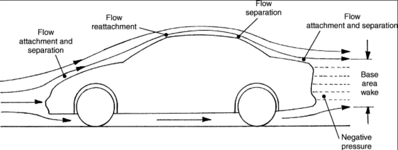
Pressure distribution across the Ahmed body and negative pressure in the wake region

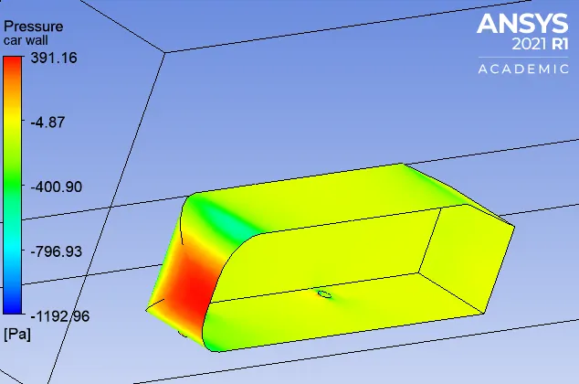
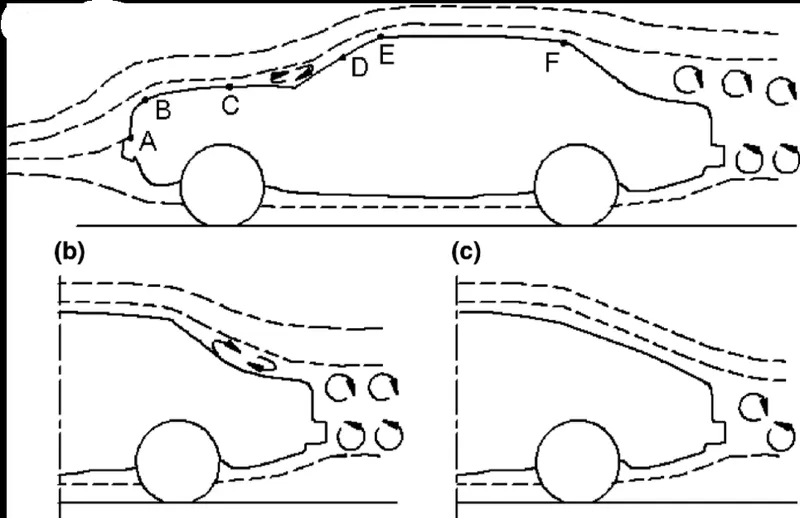
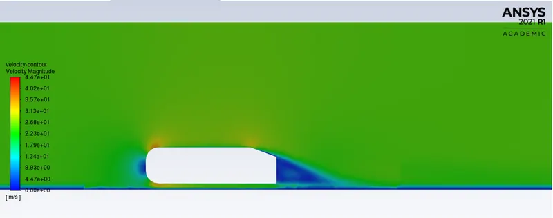
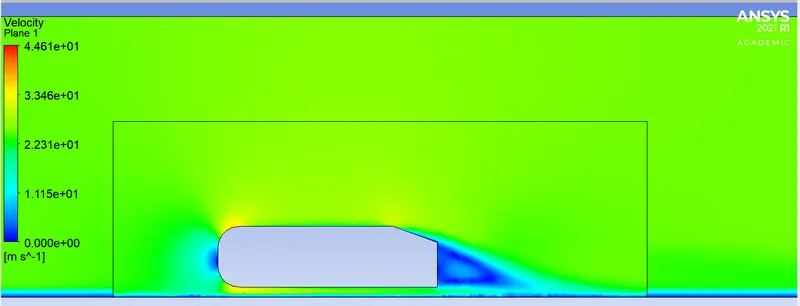
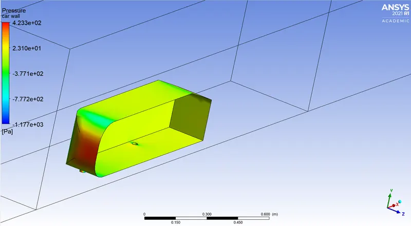
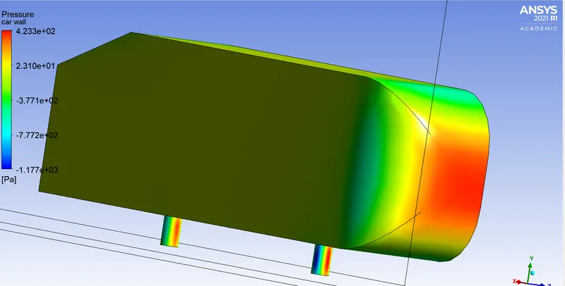
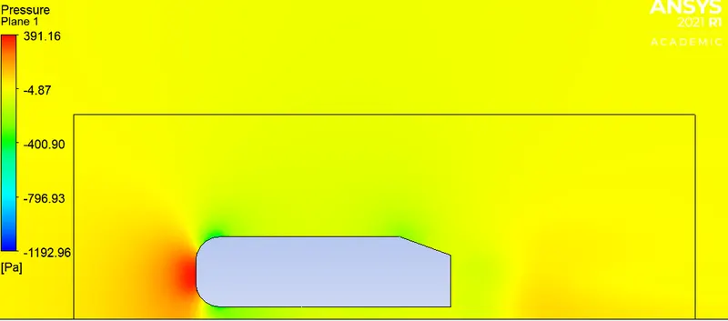
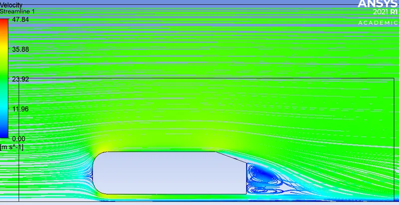
--> Pressure distribution across the Ahmed body will be shown later. As we can see, when the air flows over the surface it separates at the rear side of the Ahmed body. This creates a low-pressure turbulent region known as wake. Turbulent shear stress dominates this region. Any moving vehicle body leaves a wake region similar to the wake behind the Ahmed body. The wake contributes to pressure drag reducing vehicle performance.

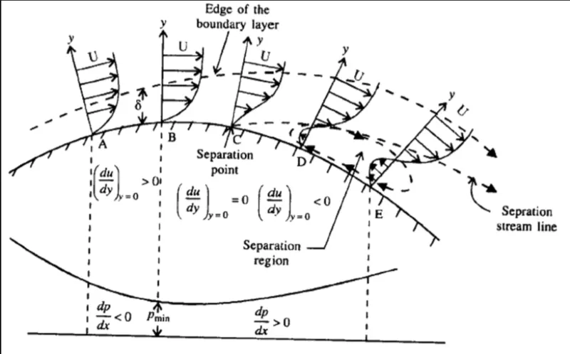
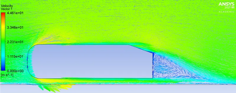
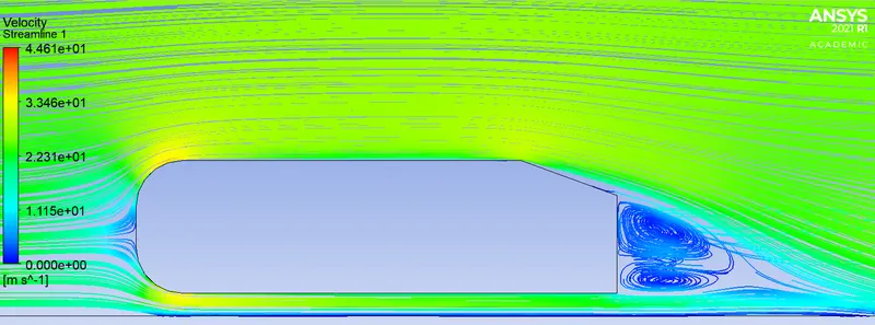
--> Because of De-acceleration near the separation region adverse pressure gradient is caused and fluid particles lose the kinetic energy and thus cannot flow downstream, causing the flow reversal and recirculation in the wake region. Detachment of the Boundary layer in the rear slant part of the Ahmed body causes a wake region with negative pressure.

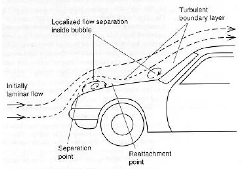
--> As we can see the front part of the Ahmed body pressure is high at the stagnation point and velocity is zero, above that the fluid accelerates and creates a small negative pressure zone on the curves in the front part. On the flat roof fluid velocity is roughly constant and pressure rises from negative to positive creating an adverse pressure gradient and a tiny localized flow separation bubble appears with separation and reattachment points.

Significance of Point of separation

--> As the flow passes through the rear part it is de-accelerated which causes increasing pressure in the flow direction, this is called the Adverse pressure gradient. There is a point close to the wall where fluid velocity reverses and the boundary layer detaches from the wall. Flow separation occurs early in the laminar flow. In the turbulent flow boundary layer is better able to remain attached to the surface and flow separation is delayed. Because of turbulent mixing momentum transfer between layers increases and hence the flow can sustain adverse pressure gradient and delay separation.

--> This idea of using turbulence to delay a flow separation in order to reduce pressure drag is also why some aeroplanes wings have small vortex generators to induce turbulence at high angle of attack to minimize the effect of flow separation. A grooved golf ball also travels farther than a smooth golf ball as turbulence delays flow seperation.

--> If we can delay flow separation, it will reduce the pressure drag force and therefore, the point of separation is important for reducing aerodynamic drag. The size of wake region is also determined by the point of separation. In the Ahmed body case, separation occurs in the rear slant part of the vehicle.

Pre-Processing

CAD Geometry

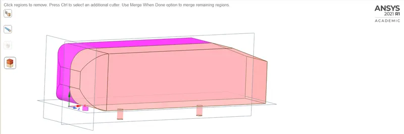
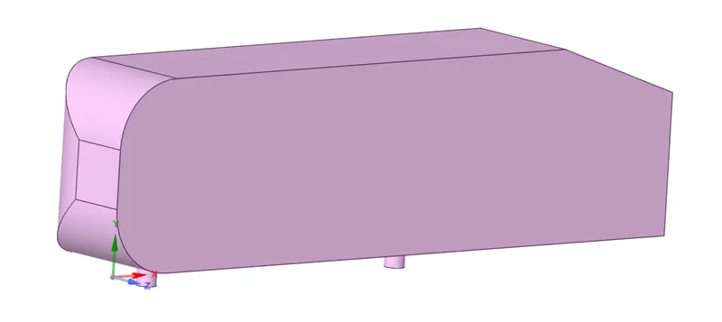
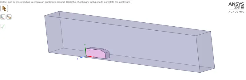
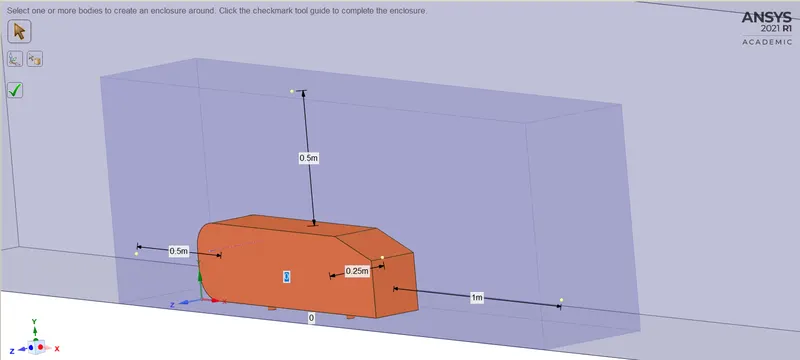
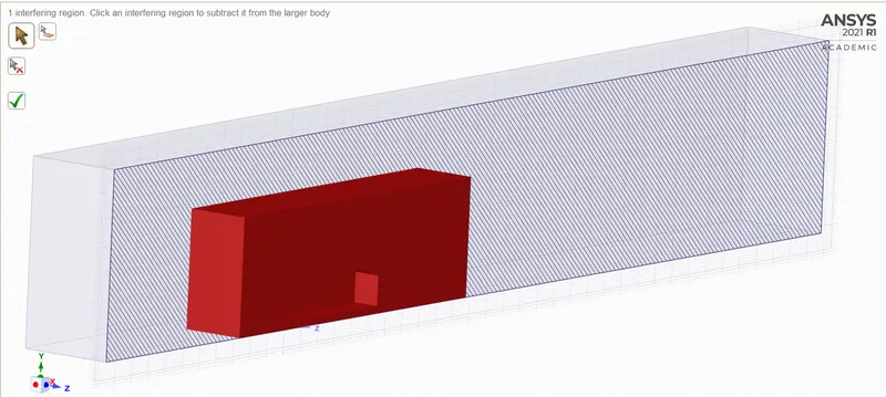
--> We need to create enclosures as shown in Ansys SpaceClaim. We have a large interference between the 2 enclosures, that we need to fix. We also have to supress the Ahmed body as we are not interested within the body. We also use the spilt body command to cut the body in half and simulate the results for half part only. We use symmetry boundary condition in the cut plane.

Spliting the body

Outer Enclosure

Inner Enclosure with Dimensions

Hatch-line pattern representing interference region.

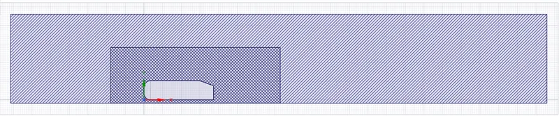
--> A particular hatch line represents an enclosure region, we can see that the inner region is represented by two hatch-line pattern. This shows that a huge interference is in this region between outer and inner enclosures.

Hatch-line pattern after fixing interference region.

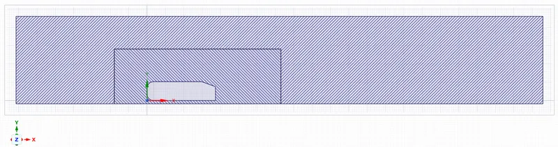
--> We can see now that after checking interference region, the inner enclosure box is represented by a single hatch pattern. Thus, interference region has been fixed.

Meshing

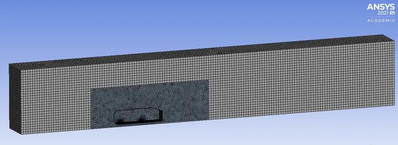
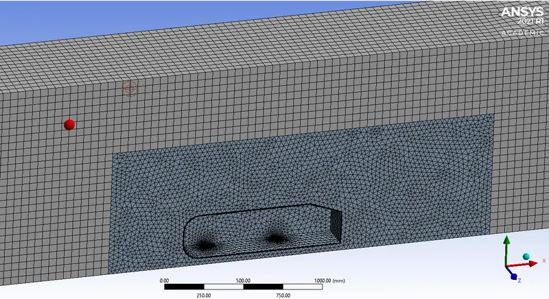
--> We use the following meshing parameters for refining the base mesh in Ansys Meshing module.

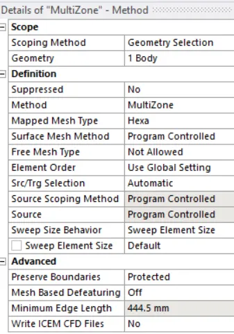
1. Multizone method on the outer enclosure box for generating hexa-hedral mesh on the outer enclosure wherever possible. Element size of the hexahedral mesh is 50 mm.

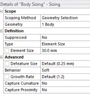
2. Body sizing parameter is also used for meshing the inner enclosure. As we want more refinement in the inner enclosure. We use tetra-hedral mesh for meshing this region. Element size is 30 mm.

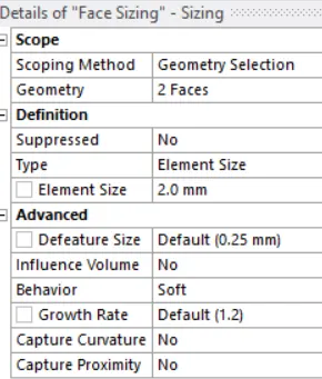
3. Face sizing parameter is imposed for controlling the mesh size on the legs of the ahmed body, a course mesh does not capture the cylindrical legs of the Ahmed body(It gives it polygonal shape). For that we need to refinr the mesh so that correct geometry is represented. Element size used for face meshing of cylindrical legs is 2 mm.

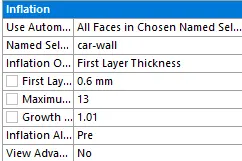
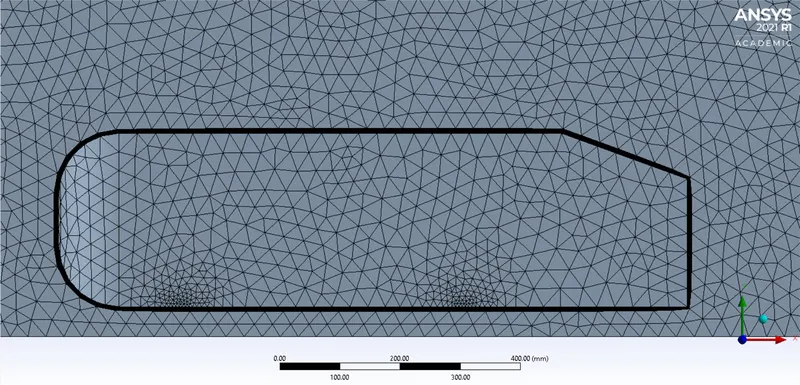
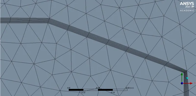
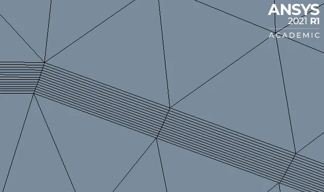
4. Finally we impose inflation layer on the car-wall for the refinement of mesh near the car wall. It is very important to add mesh refinement layers in that region, based on a value of y+ a value of first layer thickness should be used. This is related to the near wall function that is used to model the turbulent boundary layer based on some turbulence model used.

MultiZone Method body sizing method face sizing

Mesh

Mesh Near Cylindrical Legs

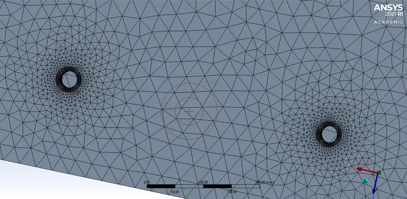
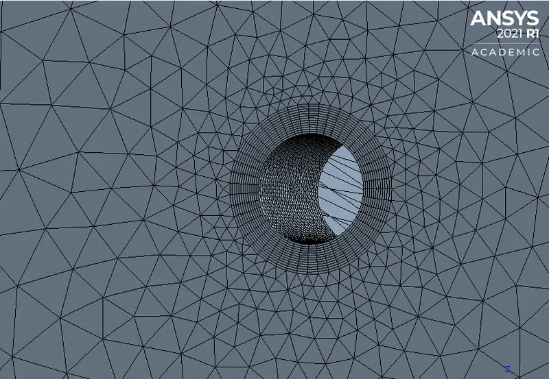
--> We can see cylindrical shape is good, mesh near faces of legs are refined and as we move away from the faces the mesh is coarse.

Car-wall Inflation Layers

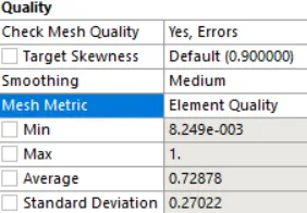
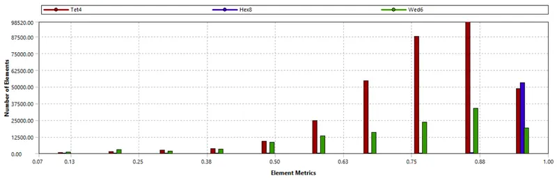
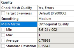
Mesh Quality

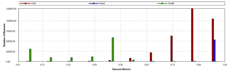
Element Quality

Orthogonal Quality

Calculation Of First Layer Thickness Of Inflation Layer

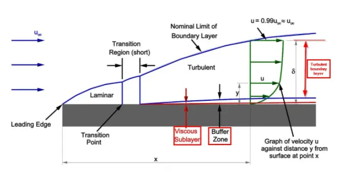
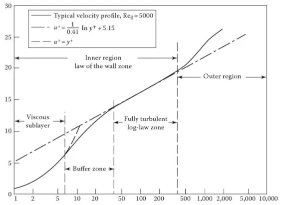
--> In order to accurately predict the flow in the boundary layer, a wall function is needed to model the boundary layer near the wall region. A turbulent boundary layer would have a very thin viscous sub-layer next to wall, a transition layer (buffer zone) and the turbulent boundary layer (log-layer). We use wall functions to resolve the flow in the viscous sub-layer and the transition layer. We keep the first mesh cell in the turbulent boundary layer or log-layer zone and employ wall function to model viscous sub-layer and buffer layer. Transition from laminar to turbulent flow is not fully understood so we cannot resolve that and therefore we model that region. In other words the first layer thickness or first mesh cell should lie in turbulent log-layer.

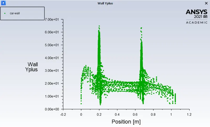
--> Another important parameter when it comes to wall functions is y-plus (y+). y+ is the non-dimensional distance from the wall to the first node from the wall. The different regions of the turbulent boundary layer based on y+ would be: laminar sub-layer (y+ <5); transition or buffer layer (5 < y+ <30); and turbulent or log-layer (y+ >30). So we need to choose y+ between 30-300 in order to keep first cell at turbulent log-layer. We choose a y+ of "42" to get first grid wall spacing as ""0.6 mm"". This will give us satisfactory results.

Post-Processing

Fluent Solver

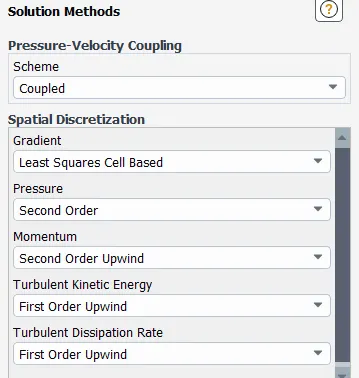
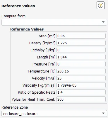
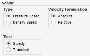
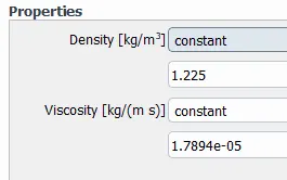
--> Fluid material used is air. The properties are shown below. Refference values are also shown below. We are using a steady pressure-based solver. For the Solution method we use coupled solver.

RESULTS

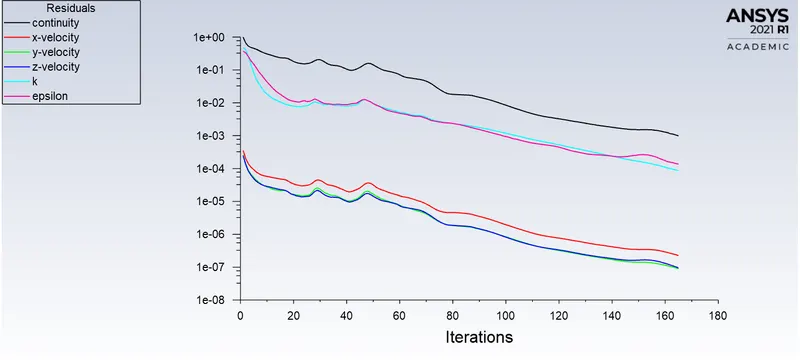
Case I -- K-ε Turbulance model with Standard wall function

Residual Plot

Velocity Contour

Pressure Contours

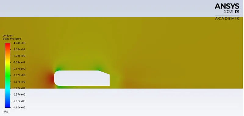
Pressure over Ahmed body

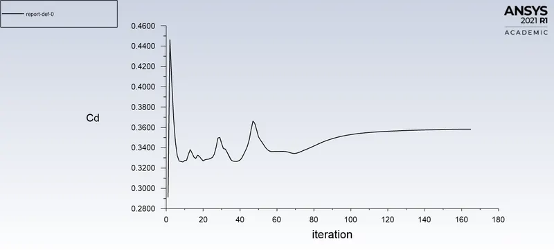
Aerodynamic Drag Coefficient

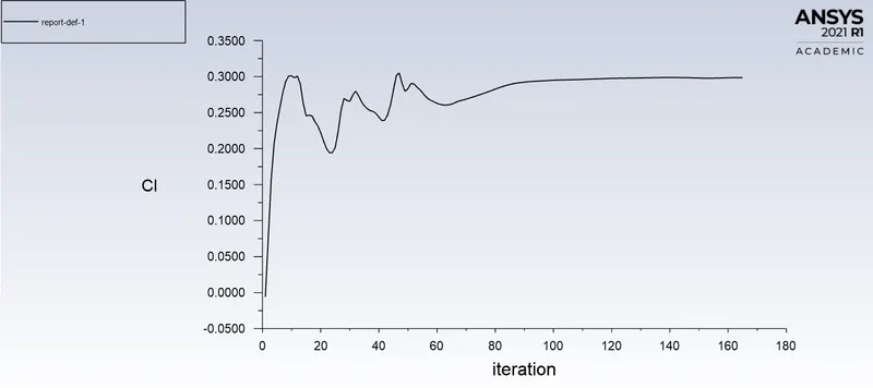
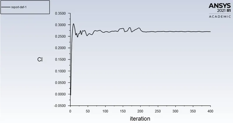
Aerodynamic Lift Coefficient

Vector Plot

Streamline Plot

Case II -- K-ω Turbulance model

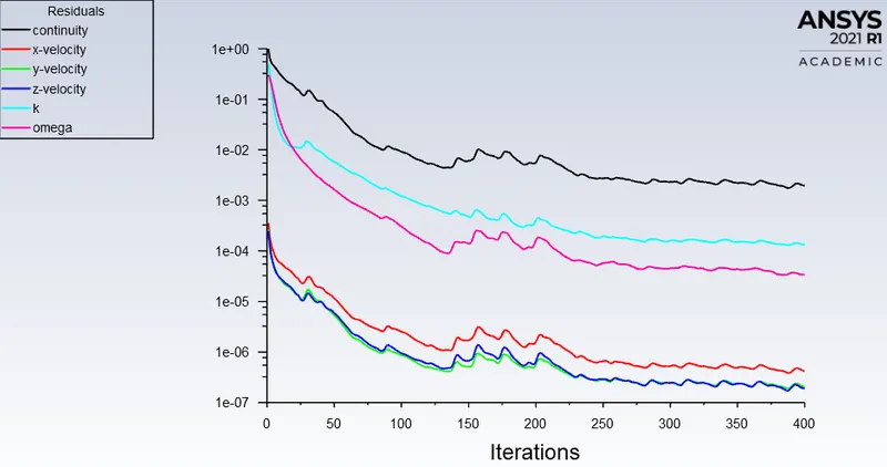
Residual Plot

Velocity Contour

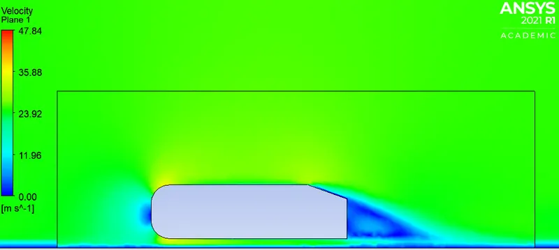
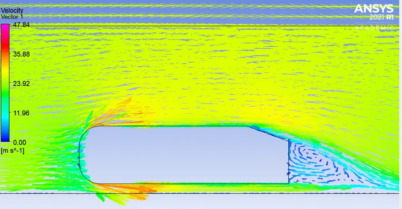
Pressure Contours

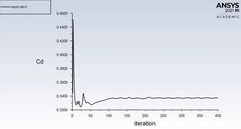
Aerodynamic Drag Coefficient

Aerodynamic Lift Coefficient

Streamlines plot

Wall y+

COMPARISON TABLE

	MESH // ELEMENTS	TURBULENCE MODEL	WALL FUNCTIONS	COEFFICIENT OF DRAG	COEFFICIENT OF LIFT
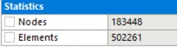
CASE I	REFINED (502261)	K-ε STANDARD	STANDARD WALL FUNCTION	0.35	0.29
CASE II	REFINED (502261)	K-ω SST	ENHANCED WALL FUNCTION	0.33	0.27

CONCLUSION

--> A coefficient of drag value of around 0.33 is what we are looking for and when we use K-ω turbulence model we get that value.

--> We can observe all the necessary aerodynamics in the flow over an Ahmed body and we also post-process some of the results.

--> Enhances wall treatment much better wall function in cases like transitional flow, separation, heat transfer, aero-dynamic drag prediction etc. The first layer for more accuracy has to be put in viscous sub-layer and for that [y+ <= 1], for complex geometries it can be up to 5.