Week 3 - External flow simulation over an Ahmed body.
AIM:- The project aims to simulate the external flow over Ahmed's body.
OBJECTIVE:- The project objective is to simulate the external flow over the Ahmed body. Here, we will perform the grid dependency test and provide the values of drag-coefficient and lift-coefficient for every case. We will also discuss-
- Ahmed's body and its importance.
- The reason for the negative pressure in the wake region.
- The significance of the point of separation.
PROJECT REPORT:- Optimized car aerodynamics is necessary to achieve efficient vehicles with minimized fuel consumption, CO2 emission, and noise while keeping good driving stability. The burning of fossil fuels becomes a more pressing issue and one main contributor to fuel burn is the car’s aerodynamic drag.
The flow region presents the major contribution to a car’s drag, which poses severe problems to numerical predictions and experimental studies as well, as the wake flow behind the car. The location at which the flow separates determines the size of the separation zone, and consequently the drag force. A more exact simulation of the wake flow and the separation process is essential for the correctness of drag predictions. However, in a real-life, the automobile is a very complex shape to model or study experimentally.
Ahmed’s body is a benchmark model widely used in the automotive industry for validating simulation tools. The Ahmed body shape is simple enough to model while maintaining car-like geometry features.
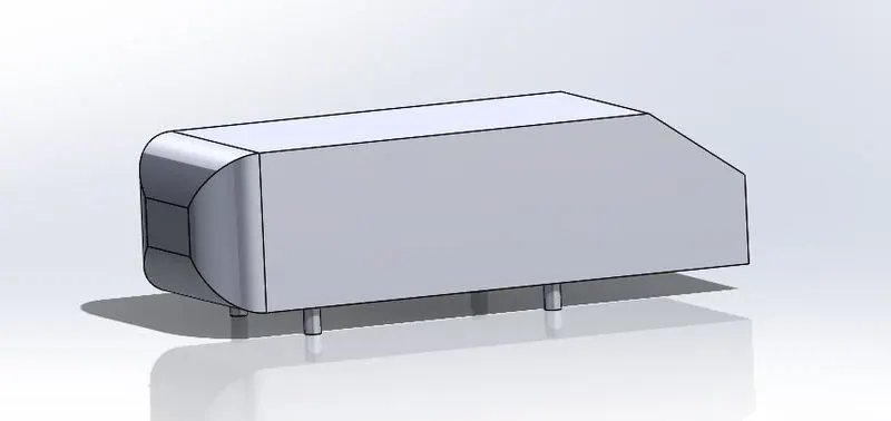
The airflow around the Ahmed body captures the essential flow features around an automobile and was first defined and characterized in the experimental work of Ahmed. Although it has a very simple shape and it allows us to capture characteristic features that are relevant to bodies in the automobile industry.
Negative pressure in the wake region:- Pressure gradient is one of the factors that influence a flow immersively. For the flat plate, the pressure gradient of the external steam is zero. But for the curved surface, upstream of the highest point, the streamlines of the outer flow converge, increasing the free stream velocity U(x) and the pressure falls with x. Downstream of the highest point the streamline diverges, resulting in a decrease of U(x) and a rise in pressure. Here, we shall investigate the effect of such pressure gradient on the shape of the boundary layer profile u(x,y). The boundary layer equation is –
`u (∂u)/(∂x)+ v (∂u)/(∂y) = -1/ρ ((∂p)/(∂x))+v (∂^2 u)/(∂y^2)`
Where the pressure gradient is found from the external velocity field as `(dp)/(dx)= -ρU((dU)/(dx))`, with x taken along the surface of the body. At the wall, the boundary layer equation becomes -
`μ((∂^2 u)/(∂y^2 ))_(wall) = (∂p)/(∂x)`
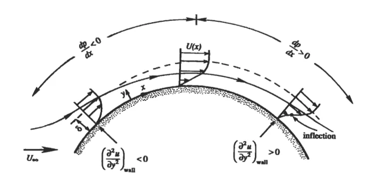
Fig:- Velocity profiles across boundary layers with favorable and adverse pressure gradients.
In an accelerating stream `(dp)/(dx)<0`, and therefore
`((∂^2 u)/(∂y^2 ))_(wall) < 0` (accelerating).
As the velocity profile has to blend in smoothly with the external profile, the slope `(∂u)/(∂y)` slightly below the edge of the boundary layer decreases with y from a positive value to zero.
In contrast, for the decelerating external stream, the curvature of the velocity profile at the wall is –
`((∂^2 u)/(∂y^2))_(wall) > 0` (decelerating).
The shape of the velocity profile in the figure suggests that a decelerating pressure tends to increase the thickness of the boundary layer. This can also be seen from the continuity equation -
`v(y)= - ∫_0^y(∂u)/(∂x) dy.`
Compared to a flat plate, a deceleration external stream causes a larger `- (∂u)/(∂x)` within the boundary layer because the deceleration of the outer flow adds to the viscous deceleration within the boundary layer. It follows from the foregoing equation that the u-field, directed away from the surface, is larger for a decelerating flow. Therefore, the boundary layer thickness is not only by the viscous diffusion but also by the advection away from the surface, resulting in a rapid increase in the boundary layer thickness with x.
If p falls along the direction of flow, `(dp)/(dx)`< 0 and we say that the pressure gradient is “favorable”. If, on the other hand, the pressure rises along the direction of flow, `(dp)/(dx)` > 0 and we say that the pressure gradient is “adverse” or “uphill”. The rapid growth of the boundary layer thickness in a decelerating stream, and the associated large v-field, causes the important phenomenon of separation, in which the external stream ceases to flow nearly parallel to the boundary surface.
Significance of the point of separation:- We see in the upper section, the boundary layer in decelerating steam has a point of inflection and grows rapidly. The existence of the point of inflection implies a slowing down of the region next to the wall, a consequence of the uphill pressure gradient. Under a strong enough adverse pressure gradient, the flow next to the wall reverses direction, resulting in a region of backward flow.
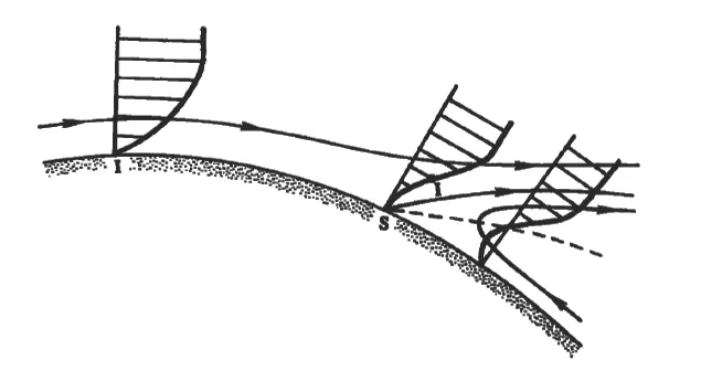
Fig:- Streamlines and velocity profiles near a separation point S. Point of inflection is indicated by I. The dashed line represents u = 0.
The reversed flow meets the forward flow at some point S at which the fluid near the surface is transported out into the mechanism. We say that the flow separates from the wall. The separation point S is defined as the boundary between the forward flow and backward flow of the fluid near the wall, where the stress vanishes -
`((∂u)/(∂y))_(wall)= 0` (separation).
It is apparent from the figure that one streamline intersects the wall at a definite angle at the point of separation.
At lower Reynolds numbers the reversed flow downstream of the point of separation forms part of a large steady vortex behind the surface (for the range of 4 < Re < 40). At higher Reynolds numbers, when the flow has boundary layer characteristics, the flow downstream of separation is unsteady and frequently chaotic.
How strong an adverse pressure gradient the boundary layer can withstand without undergoing separation depends on the geometry of flow, and whether the boundary layer is laminar or turbulent. A steep pressure gradient, such as that behind a blunt body, invariably leads to a quick separation. In contrast, the boundary layer on the trailing surface of a thin body can overcome the weak pressure gradient involved. Therefore, to avoid separation and large drag, the trailing section of a submerged body should be gradually reduced in size, and it calls a streamlined shape.
The point of separation is insensitive to the Reynolds number as long as the boundary layer is laminar. But when the flow is going towards the transition to turbulence flow, which delays boundary layer separation. A turbulent boundary layer is more capable of withstanding an adverse pressure gradient. This is because the velocity profile is a turbulent boundary layer that is “fuller” and has more energy.
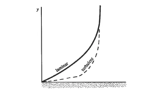
Fig:- Comparison of laminar and turbulent velocity profile in a boundary layer.
Now we start our simulation. Here, we do grid dependancy test and so we start observe our result for the case of corse meshing and then for the medium and next for the fine mesh. The air velocity which flows over the Ahamed body is 25 m/s and the temperature is 300k. Here we perform k-epsilon and k-omega model for each coarse, medium, and fine case.
Steps to run the simulation:-We simulate the flow in fluent by following those steps:-
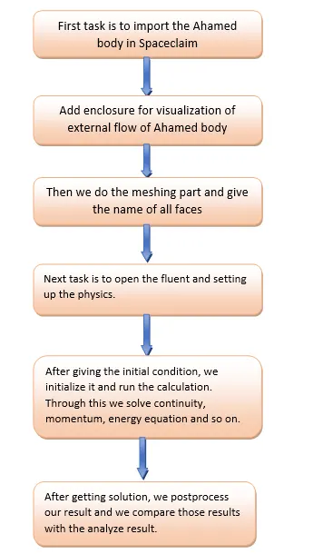
Simulation for Coarse meshing:-
Case_1:- K-epsilon model
Geometry:-
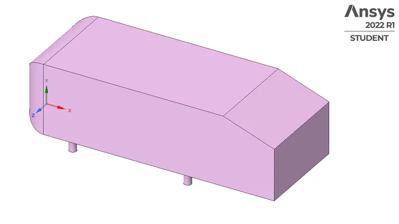
The Ahamed body:-
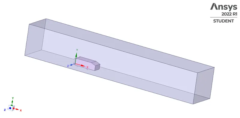
Adding enclosure:- For visualizing external flow, we need to add enclosure
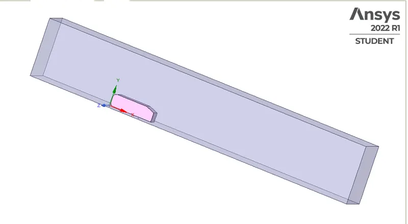
Splitting body:- As the body is perfectly symmetric, we can run the simulation by considering the only half body. This is the best practice where you can save on the number of cells and get the results faster as well
Meshing:-
The geometry is prepared and now we go for meshing part:-
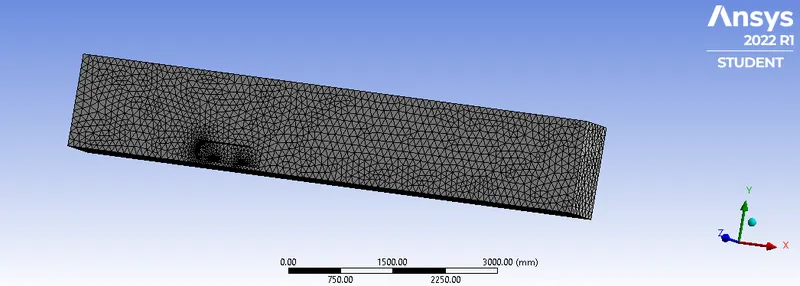
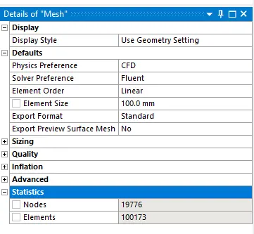
Mesh Information for Fluid Flow using k epsilon method:-
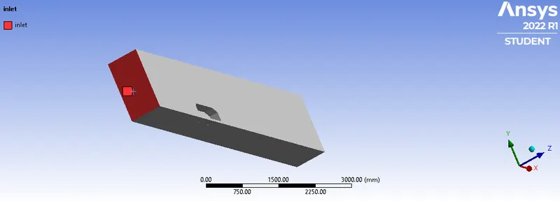
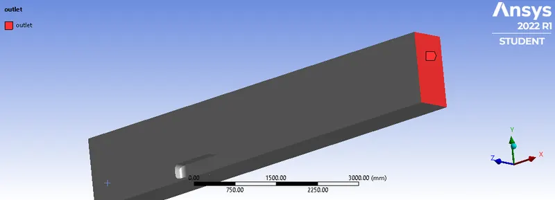
Specify the each face name:-
Inlet:-
Outlet:-
Symmetry wall:-
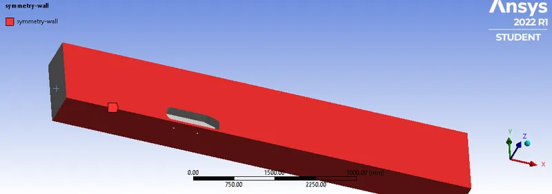
Car wall:-
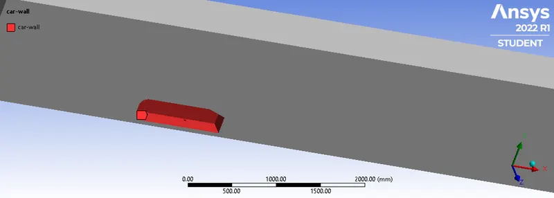
Setting up the physics in fluent:-
Models
------

   Model                        Settings
   ----------------------------------------------------------------
   Space                        3D
   Time                         Steady
   Viscous                      Standard k-epsilon turbulence model
   Wall Treatment               Standard Wall Functions
   Heat Transfer                Enabled
   Solidification and Melting   Disabled
   Radiation                    None
   Species                      Disabled
   Coupled Dispersed Phase      Disabled
   NOx Pollutants               Disabled
   SOx Pollutants               Disabled
   Soot                         Disabled
   Mercury Pollutants           Disabled
   Structure                    Disabled
   Acoustics                    Disabled
   Eulerian Wall Film           Disabled
   Potential/Li-ion Battery     Disabled
   Multiphase                   Disabled


Material Properties
-------------------

   Material: air (fluid)

      Property                        Units      Method     Value(s)
      ----------------------------------------------------------------
      Density                         kg/m^3     constant   1.225
      Cp (Specific Heat)              J/(kg K)   constant   1006.43
      Thermal Conductivity            W/(m K)    constant   0.0242
      Viscosity                       kg/(m s)   constant   1.7894e-05
      Molecular Weight                kg/kmol    constant   28.966
      Thermal Expansion Coefficient   K^-1       constant   0
      Speed of Sound                  m/s        none       #f

   Material: aluminum (solid)

      Property               Units      Method     Value(s)
      -----------------------------------------------------
      Density                kg/m^3     constant   2719
      Cp (Specific Heat)     J/(kg K)   constant   871
      Thermal Conductivity   W/(m K)    constant   202.4


Cell Zone Conditions
--------------------

   Zones

      name                  id   type
      --------------------------------
      enclosure_enclosure   2    fluid

   Setup Conditions

      enclosure_enclosure

         Condition       Value
         ---------------------
         Frame Motion?   no


Boundary Conditions
-------------------

   Zones

      name            id   type
      ------------------------------------
      outlet          5    pressure-outlet
      symmetry-wall   6    symmetry
      car-wall        7    wall
      inlet           8    velocity-inlet

   Setup Conditions

      outlet

         Condition   Value
         -----------------

      symmetry-wall

         Condition   Value
         -----------------

      car-wall

         Condition                  Value
         ------------------------------------------
         Thermal BC Type            Heat Flux
         Wall Motion                Stationary Wall
         Shear Boundary Condition   No Slip

      inlet

         Condition                  Value
         --------------------------------
         Velocity Magnitude [m/s]   25


Solver Settings
---------------

   Equations

      Equation     Solved
      -------------------
      Flow         yes
      Turbulence   yes
      Energy       yes

   Numerics

      Numeric                         Enabled
      ---------------------------------------
      Absolute Velocity Formulation   yes

   Pseudo Time Explicit Relaxation Factors

      Variable                     Relaxation Factor
      ----------------------------------------------
      Density                      1
      Body Forces                  1
      Turbulent Kinetic Energy     0.75
      Turbulent Dissipation Rate   0.75
      Turbulent Viscosity          1
      Energy                       0.75
      Explicit Momentum            0.5
      Explicit Pressure            0.5

   Linear Solver

      Variable                     Solver Type   Termination Criterion   Residual Reduction Tolerance
      -----------------------------------------------------------------------------------------------
      Flow                         F-Cycle       0.1
      Turbulent Kinetic Energy     F-Cycle       0.1
      Turbulent Dissipation Rate   F-Cycle       0.1
      Energy                       F-Cycle       0.1

   Pressure-Velocity Coupling

      Parameter                               Value
      -----------------------------------------------
      Type                                    Coupled
      Pseudo Time Method (Global Time Step)   yes

   Discretization Scheme

      Variable                     Scheme
      ------------------------------------------------
      Pressure                     Second Order
      Momentum                     Second Order Upwind
      Turbulent Kinetic Energy     First Order Upwind
      Turbulent Dissipation Rate   First Order Upwind
      Energy                       Second Order Upwind

   Solution Limits

      Quantity                         Limit
      ---------------------------------------
      Minimum Absolute Pressure        1
      Maximum Absolute Pressure        5e+10
      Minimum Temperature              1
      Maximum Temperature              5000
      Minimum Turb. Kinetic Energy     1e-14
      Minimum Turb. Dissipation Rate   1e-20
      Maximum Turb. Viscosity Ratio    100000
Results:-
Residuals:-
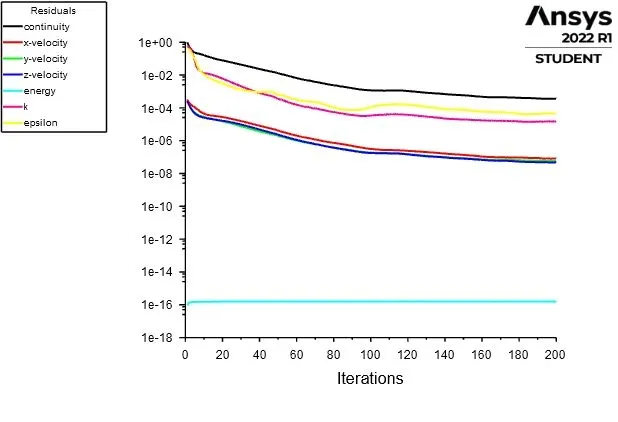
Drag Coefficient:- In this case drag coefficient value is 0.385
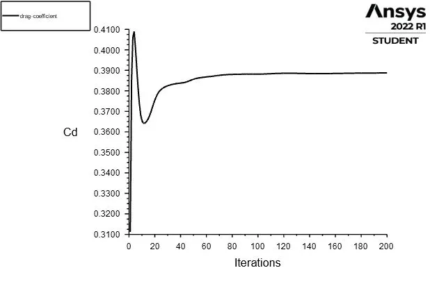
Lift Coefficient:- In this case the lift coefficient value is 0.27
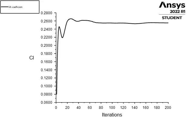
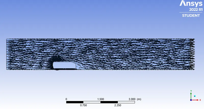
Vector Plot on the cut plane:-
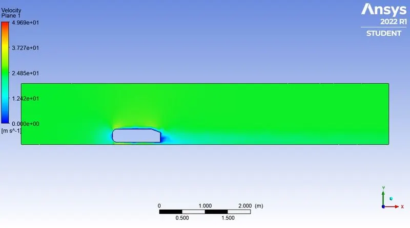
Velocity contour Plot on the cut plane:-
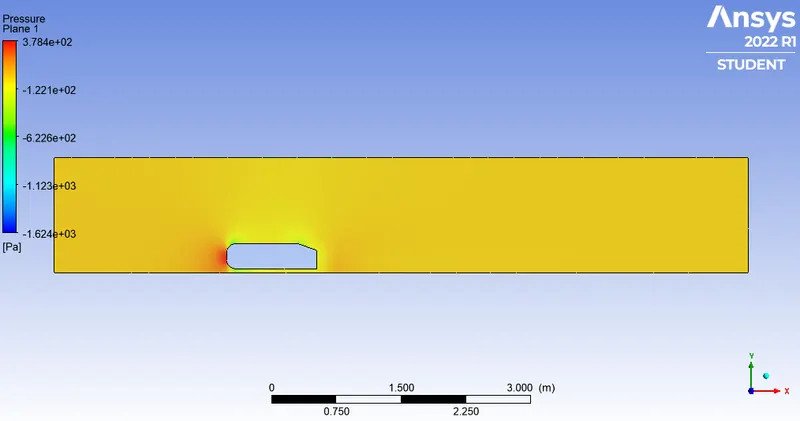
Pressure contour Plot on the cut plane:-
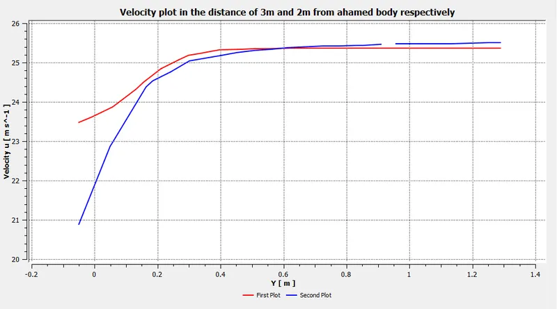
Velocity line plot:-
Case 2:- K-omega model
In this case all procedures are same just instead of taking k-epsilon model, we take k-omega sst model.
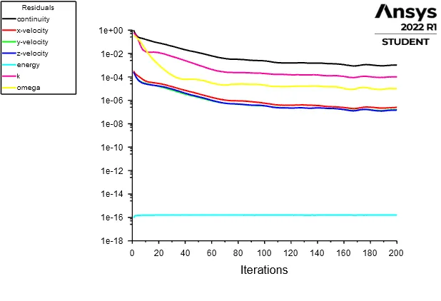
Residual:-
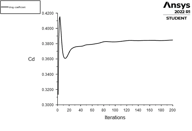
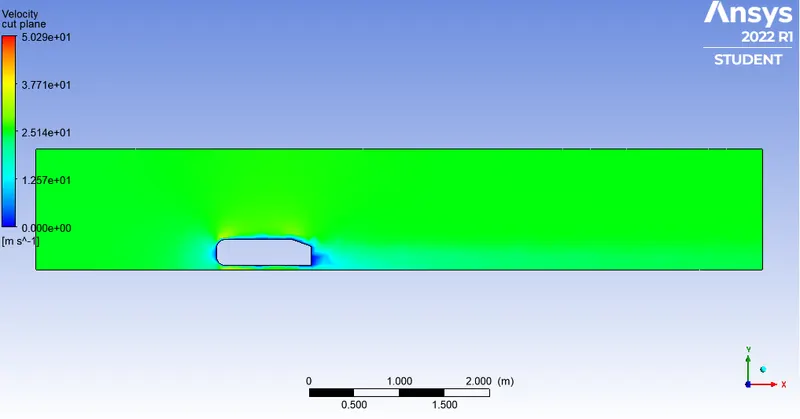
Drag Coefficient:- In this case the drag coefficient value is 0.383
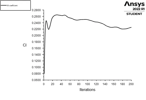
Lift Coefficient:- In this case the lift coefficient value is 0.2256
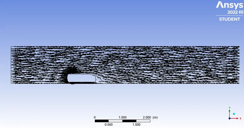
Vector Plot on the cut plane:-
Velocity contour Plot on the cut plane:-
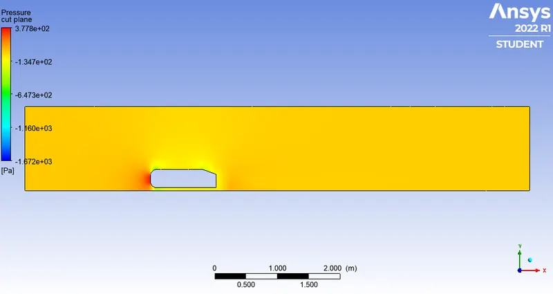
Pressure contour Plot on the cut plane:-
Velocity line plot
Simulation for Medium meshing:- Here we add two enclosures because we need more cells near the Ahamed body. So we need an enclosure near the Ahamed body. That's how we can capture more physics phenomena near the Ahamed body.
The Ahamed body:-
Adding first enclosure:-
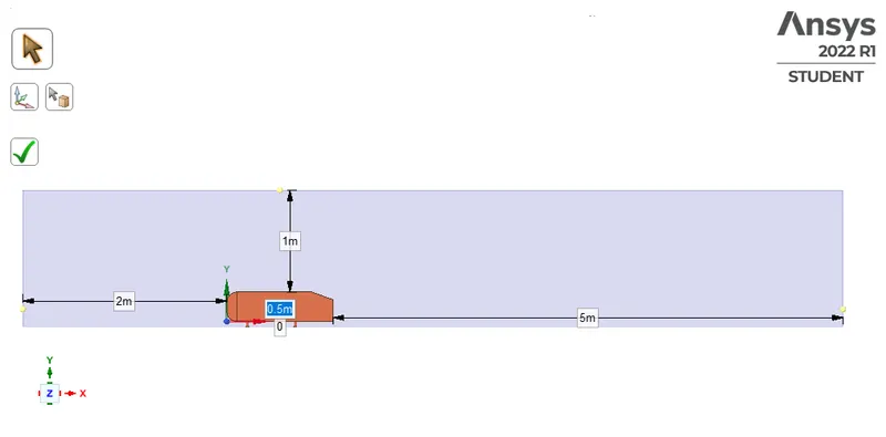
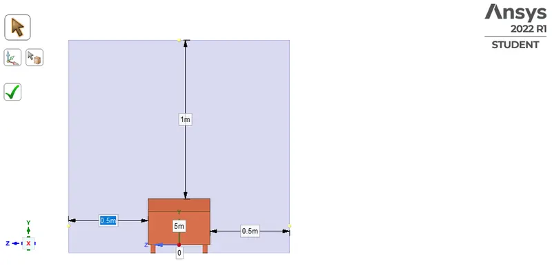
Adding second enclosure:-
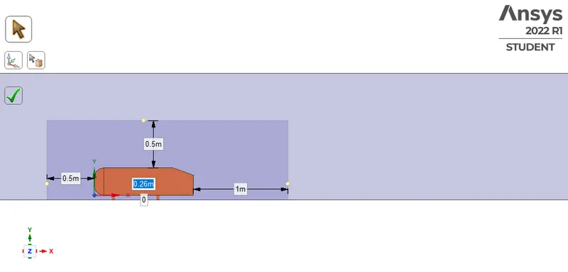
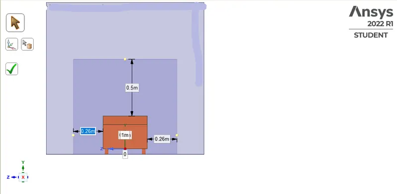
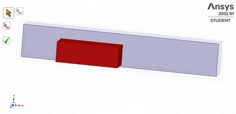
Removing Interference:- We create hatches in a side cut plane. Each section have different hatch pattern. If we see the below picture carefully, the hatch inside our smaller box contains hatches from both side that means it is an overlapping regeion and we don't want that.
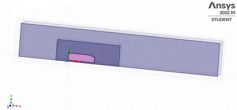
Now, if we go to prepare geometry and run the interference check then SpaceClaim able to say that in the inner box there is a huge interference.
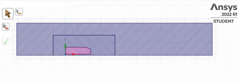
After removing interference it looks like
Splitting body:- As the body is perfectly symmetric, we can run the simulation by considering the only half body. This is the best practice where we can save on the number of cells and get the results faster as well
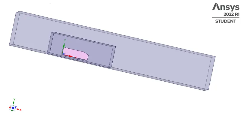
Now for the two blocks that are sharing the information, we use share topology. We go for meshing now.
Meshing:-
MultiZone Method:- The MultiZone mesh method provides automatic decomposition of geometry into mapped (structured/sweepable) regions and free (unstructured) regions. It automatically generates a pure hexahedral mesh where possible and then fills the more difficult to capture regions with unstructured mesh.So here we first use Multizone method and the element size is 100mm.
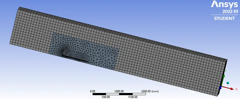
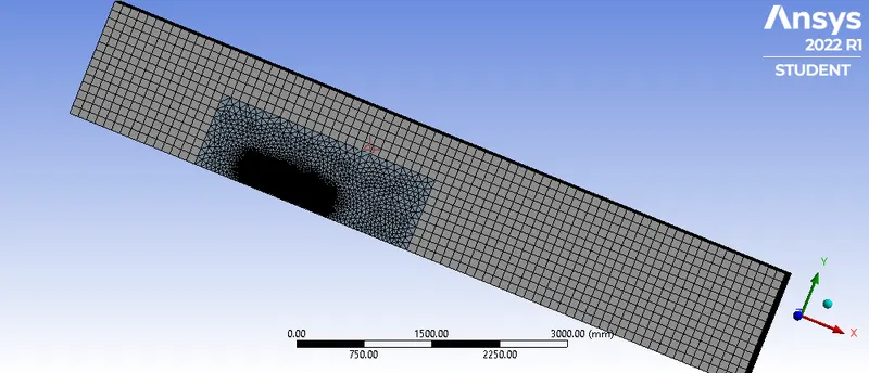
Body xizing:-Then we increase the elements of the smaller box to capture how fluid flows in the wake region. We give the element sixe 50mm.
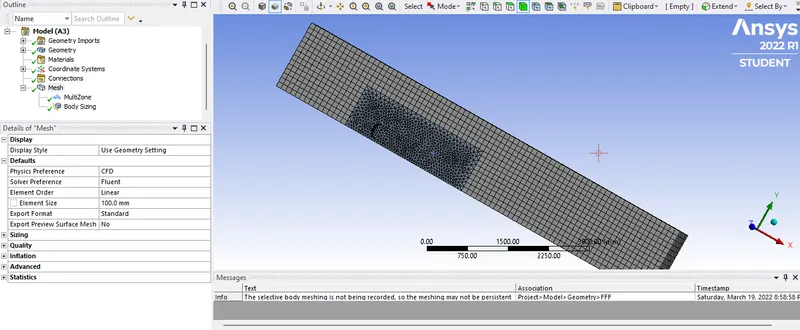
Face sizing:- After that we increase the car wall element. We just select the car wall faces and insert the sizing method and give the element sixe 10mm.
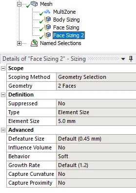
Face sizing2:- If we see the cylindrical surface or cylindrical pillar that supports the Ahamed body, they are approximated as polygons. The cylindrical surface’s element size is quite big in this case.
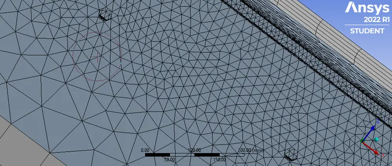
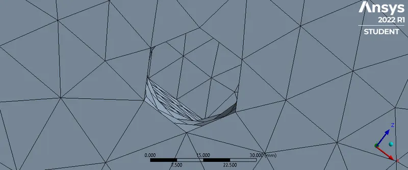
So we should decrease the element size to make it as a circle.So we select the cylindrical pillar and we give the element size 5mm.
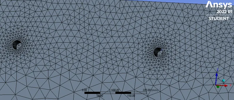
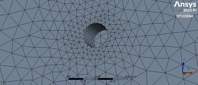
Inflation Layer:-Now we can see the outside of the car wall, each cell has the center point in a different location which is not ideal for applying boundary conditions. Because for each boundary we need to specify the boundary condition.
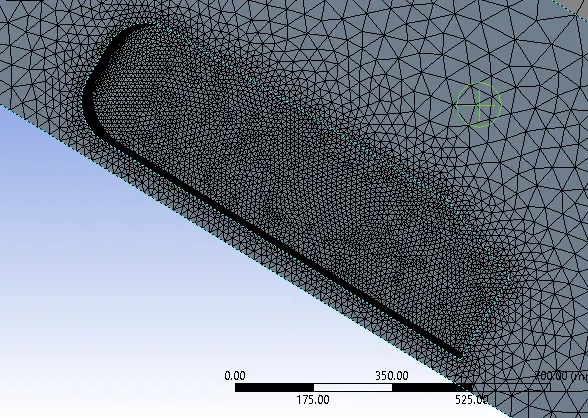
So, we want to create a set of cells that follow the shape of a surface quite closely these are called the inflation layer. So first we go to mesh, then go to inflation, choose All faces in chosen Named selection, after that choose the car wall name, and we use first layer thickness. The first layer thickness is 5mm which we have to define.
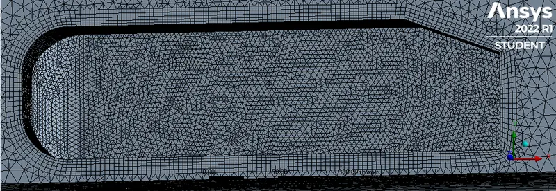
If we see the inflation layer carefully we see that they are irregular and thicknesses are varying in many places. So instead of going first layer thickness, we go for total thickness. If the first layer thickness is 5, the growth rate is 1.2, and we do 5 inflation layers, so our total thickness is 5*(1.2^5) = 12.5. After generating mesh we see that the inflation layer is much better and much more regular and that’s because we are providing the total thickness which is going to constrain the mesh in the right direction.
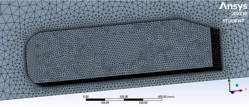
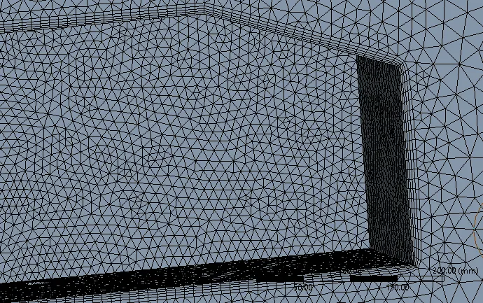
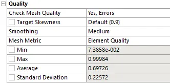
The mesh details are:-
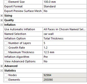
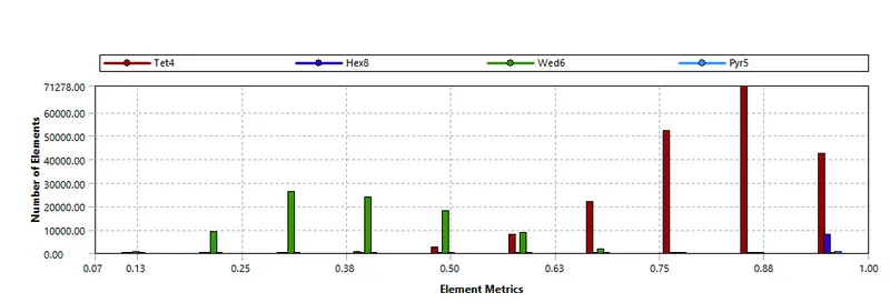
Check Mesh Quality:-
Named Selection:-
Inlet:-
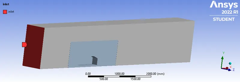
Outlet:-
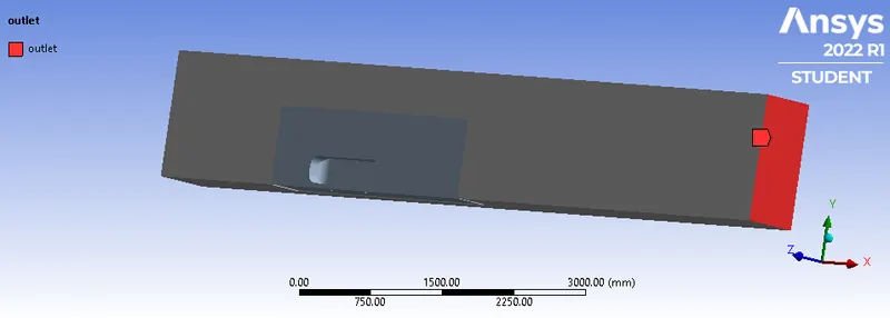
Symmetry Wall:-
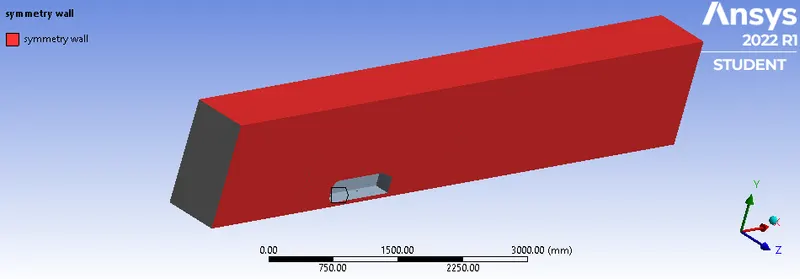
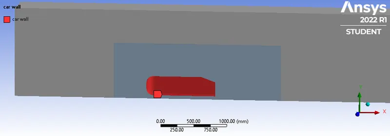
Car Wall:-
Case_1:- K-epsilon model
Setting up the Physics:-
Models
------

   Model                        Settings
   ----------------------------------------------------------------
   Space                        3D
   Time                         Steady
   Viscous                      Standard k-epsilon turbulence model
   Wall Treatment               Standard Wall Functions
   Heat Transfer                Enabled
   Solidification and Melting   Disabled
   Radiation                    None
   Species                      Disabled
   Coupled Dispersed Phase      Disabled
   NOx Pollutants               Disabled
   SOx Pollutants               Disabled
   Soot                         Disabled
   Mercury Pollutants           Disabled
   Structure                    Disabled
   Acoustics                    Disabled
   Eulerian Wall Film           Disabled
   Potential/Li-ion Battery     Disabled
   Multiphase                   Disabled


Material Properties
-------------------

   Material: air (fluid)

      Property                        Units      Method     Value(s)
      ----------------------------------------------------------------
      Density                         kg/m^3     constant   1.225
      Cp (Specific Heat)              J/(kg K)   constant   1006.43
      Thermal Conductivity            W/(m K)    constant   0.0242
      Viscosity                       kg/(m s)   constant   1.7894e-05
      Molecular Weight                kg/kmol    constant   28.966
      Thermal Expansion Coefficient   K^-1       constant   0
      Speed of Sound                  m/s        none       #f

   Material: aluminum (solid)

      Property               Units      Method     Value(s)
      -----------------------------------------------------
      Density                kg/m^3     constant   2719
      Cp (Specific Heat)     J/(kg K)   constant   871
      Thermal Conductivity   W/(m K)    constant   202.4


Cell Zone Conditions
--------------------

   Zones

      name                      id   type
      ------------------------------------
      fff-enclosure_enclosure   2    fluid

   Setup Conditions

      fff-enclosure_enclosure

         Condition       Value
         ---------------------
         Frame Motion?   no


Boundary Conditions
-------------------

   Zones

      name            id   type
      ------------------------------------
      car_wall        5    wall
      symmetry_wall   6    symmetry
      inlet           7    velocity-inlet
      outlet          8    pressure-outlet

   Setup Conditions

      car_wall

         Condition                  Value
         ------------------------------------------
         Thermal BC Type            Heat Flux
         Wall Motion                Stationary Wall
         Shear Boundary Condition   No Slip

      symmetry_wall

         Condition   Value
         -----------------

      inlet

         Condition                  Value
         --------------------------------
         Velocity Magnitude [m/s]   25

      outlet

         Condition   Value
         -----------------

Solver Settings
---------------

   Equations

      Equation     Solved
      -------------------
      Flow         yes
      Turbulence   yes
      Energy       yes

   Numerics

      Numeric                         Enabled
      ---------------------------------------
      Absolute Velocity Formulation   yes

   Pseudo Time Explicit Relaxation Factors

      Variable                     Relaxation Factor
      ----------------------------------------------
      Density                      1
      Body Forces                  1
      Turbulent Kinetic Energy     0.75
      Turbulent Dissipation Rate   0.75
      Turbulent Viscosity          1
      Energy                       0.75
      Explicit Momentum            0.5
      Explicit Pressure            0.5

   Linear Solver

      Variable                     Solver Type   Termination Criterion   Residual Reduction Tolerance
      -----------------------------------------------------------------------------------------------
      Flow                         F-Cycle       0.1
      Turbulent Kinetic Energy     F-Cycle       0.1
      Turbulent Dissipation Rate   F-Cycle       0.1
      Energy                       F-Cycle       0.1

   Pressure-Velocity Coupling

      Parameter                               Value
      -----------------------------------------------
      Type                                    Coupled
      Pseudo Time Method (Global Time Step)   yes

   Discretization Scheme

      Variable                     Scheme
      ------------------------------------------------
      Pressure                     Second Order
      Momentum                     Second Order Upwind
      Turbulent Kinetic Energy     First Order Upwind
      Turbulent Dissipation Rate   First Order Upwind
      Energy                       Second Order Upwind

   Solution Limits

      Quantity                         Limit
      ---------------------------------------
      Minimum Absolute Pressure        1
      Maximum Absolute Pressure        5e+10
      Minimum Temperature              1
      Maximum Temperature              5000
      Minimum Turb. Kinetic Energy     1e-14
      Minimum Turb. Dissipation Rate   1e-20
      Maximum Turb. Viscosity Ratio    100000
Results:-
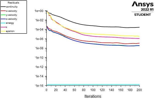
Residual:-
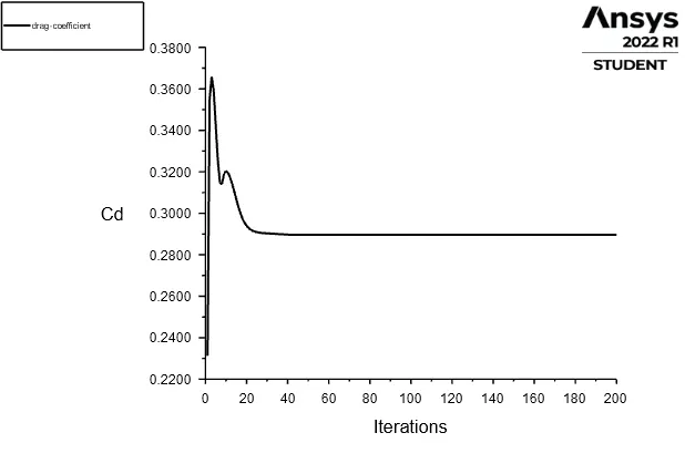
Drag Coefficient:- The value of Drag coefficient is 0.29.
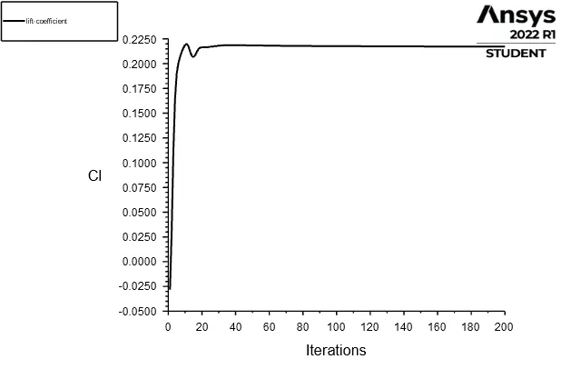
Lift Coefficient:- The value of lift coefficient is 0.225.
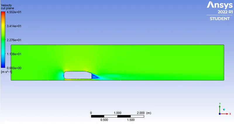
Velocity Contour Plot on Cut Plane:-
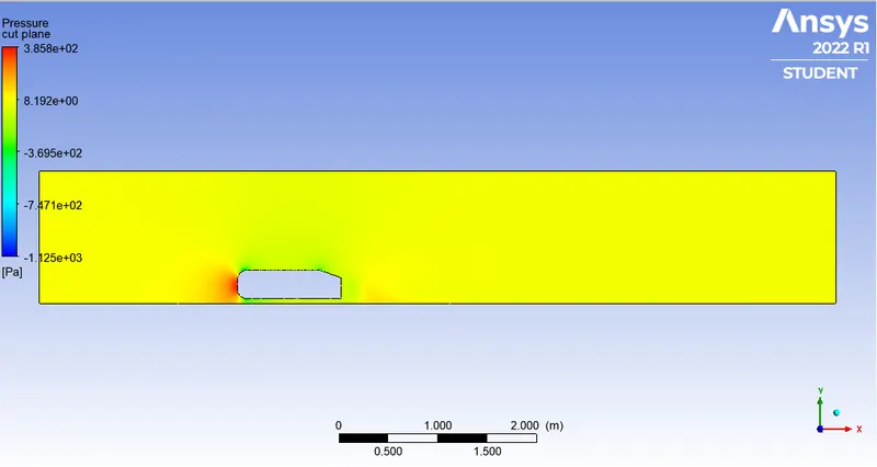
Pressure Contour Plot on Cut Plane:-
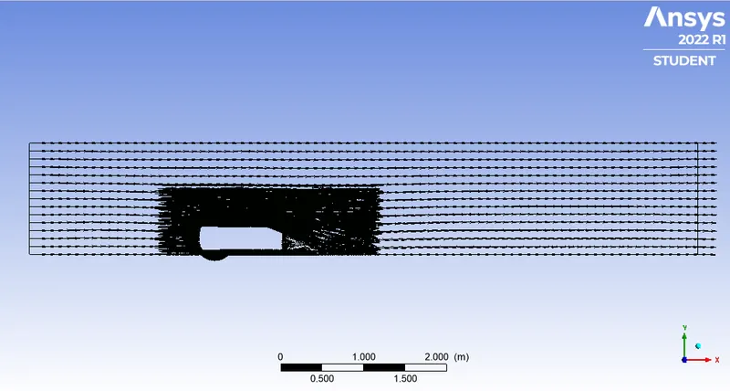
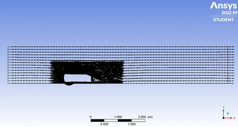
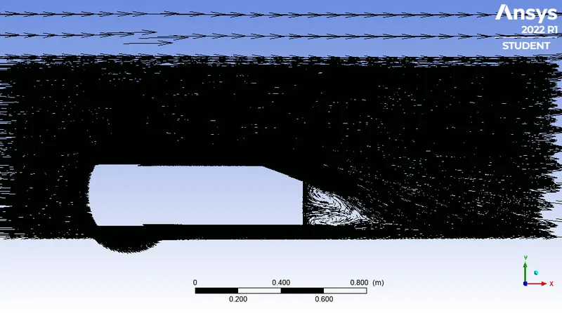
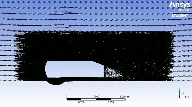
Vector Plot on cut plane:- A vector plot is a qualitative representation of spatial magnitude. The only limitation is that it can be drawn plane or a 3D twisted surface. It is helping us to visualize the flow field. Here it is very nicely seen how the fluid flows over the Ahamed body.
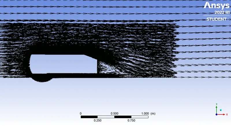
If we zoom on the wake region portion then we can see that for a very small area in the wake region the fluid path is a squirrel.
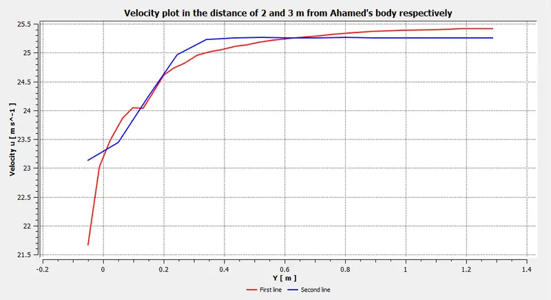
Velocity line plot:-
Case_2:- K-omega model
Results:-
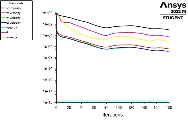
Residual:-
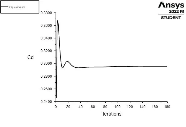
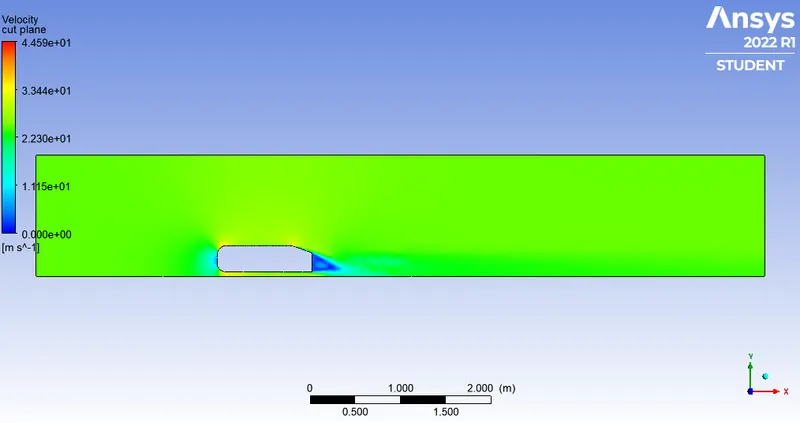
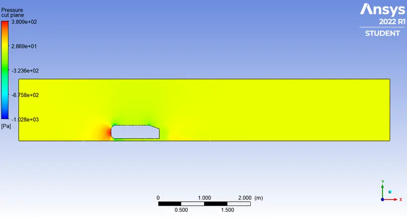
Drag Coefficient:- Here the value of Drag coefficient is approx 0.29.
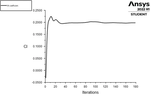
Lift Coefficient:- Here the value of lift coefficient is approx 0.2.
Velocity Contour Plot on cut plane:-
Pressure Contour Plot on cut plane:-
Vector plot on cut plane:-
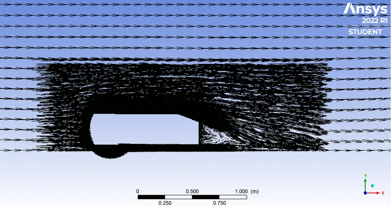
Velocity line plot:-
Simulation for Finer meshing:- Here we follow all the . All those processes are same as medium meshing. Just we increase the elements to 449577 in meshing.
Details of meshing:-
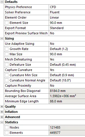
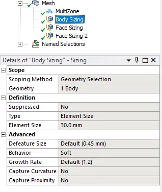
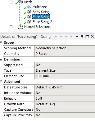
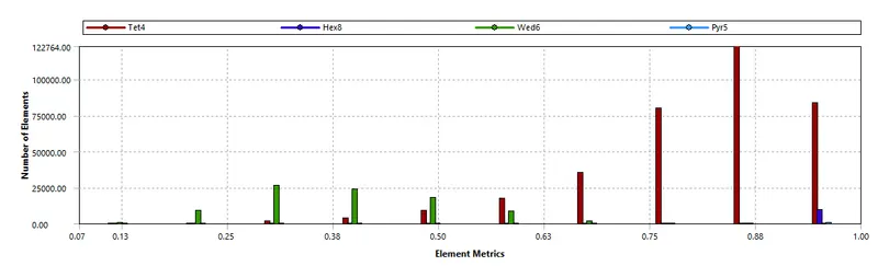
Quality check of meshing:-
Now we go for solution part of this simulation.
Case_1:- K-epsilon model
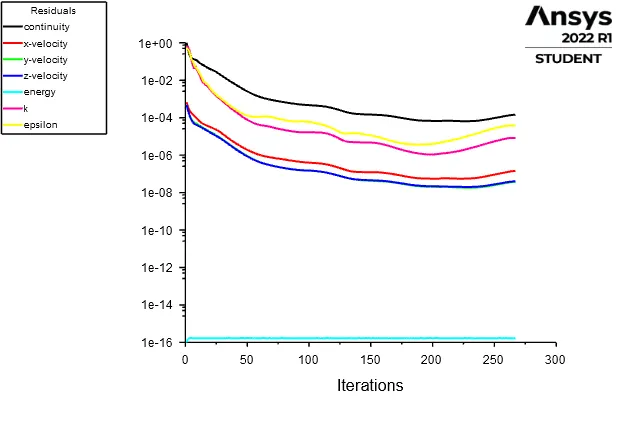
Residual:-
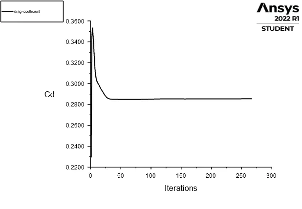
Drag Coefficient:- Here the value of Drag coefficient is approx 0.287.
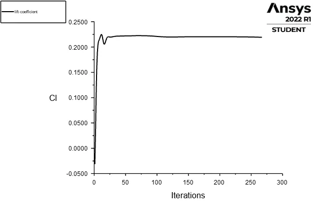
Lift Coefficient:- Here the value of Lift coefficient is approx 0.224.
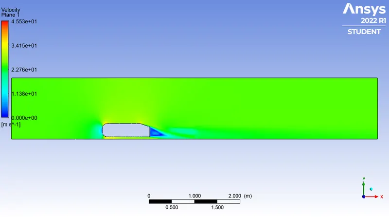
Velocity Contour Plot on cut plane:-
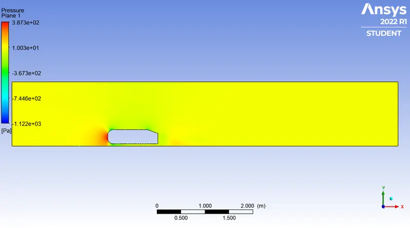
Pressure Contour Plot on cut plane:-
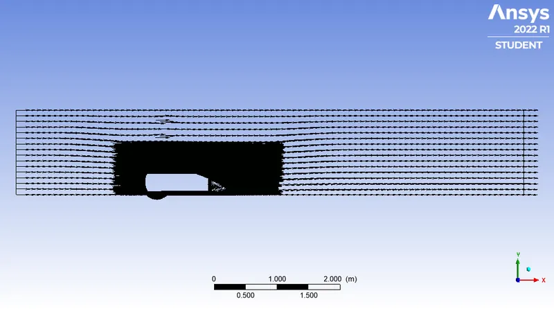
Vector Plot:-
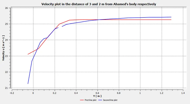
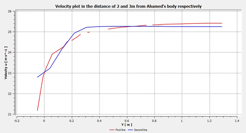
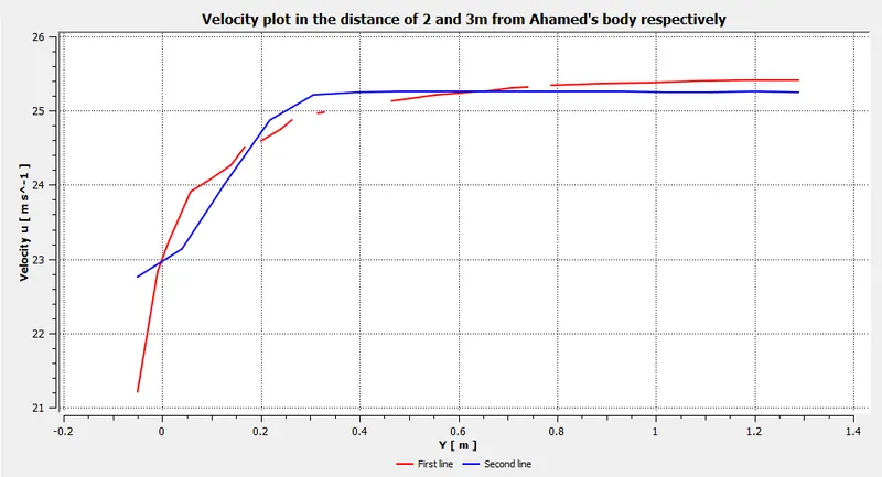
Velocity line plot:- First line is discontinuous because there some data is unavailable.
Case_2:- K-omega model
In this case whole procedure is same as case_1 for medium meshing. The only difference is that here we choose K-omega sst model. So, we just focus on our results.
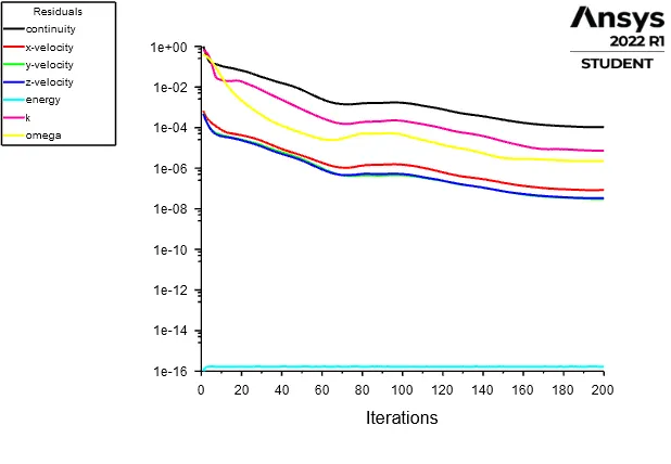
Residual:-
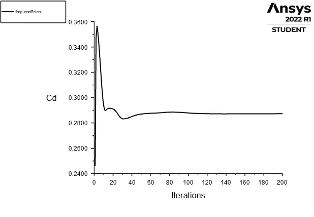
Drag Coefficient:- Here the value of Drag coefficient is approx 0.287.
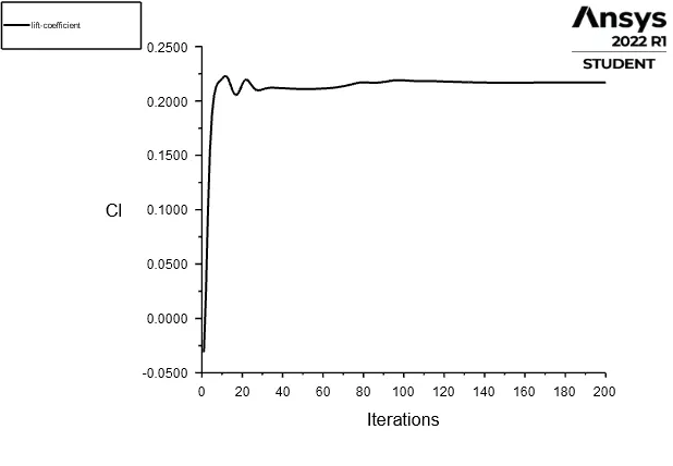
Lift Coefficient:- Here the value of lift coefficient is approx 0.224.
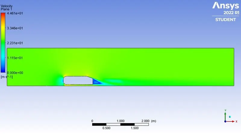
Velocity Contour Plot on cut plane:-
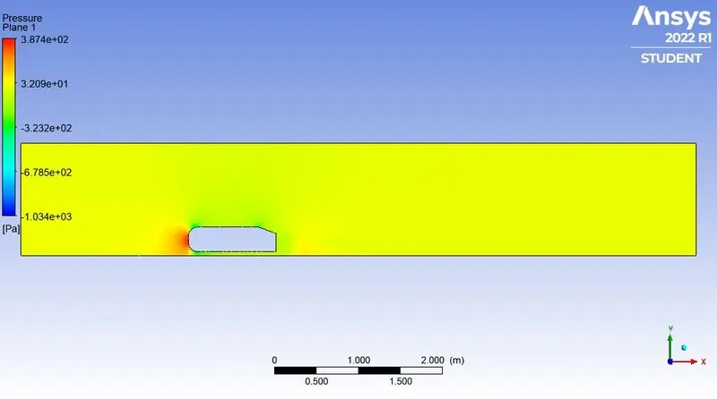
Pressure Contour Plot on cut plane:-
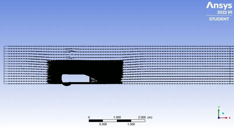
Vector plot on cut plane:-
Velocity line plot:- First line is discontinuous because there some data is unavailable.
OBSERVATION TABLE:-
| Type of meshing based on their elements number | Drag Coefficient | Lift Coefficient |
| Coarse Meshing | 0.383 | 0.2256 |
| Medium Meshing | 0.29 | 0.225 |
| Fine Meshing | 0.287 | 0.224 |
CONCLUSION:-
- We see that except for the frontside of Ahamed’s body (which faces the flow), in every place, there is a negative pressure gradient. And a negative pressure gradient helps us to suppress the separation and reduce the drag coefficient. So it is a good sign for our geometry.
- We use turbulent flow in our case. Because it delays the boundary layer separation. A turbulent boundary layer is more capable of withstanding an adverse pressure gradient. This is because the velocity profile is a turbulent boundary layer that is “fuller” and has more energy.
- To avoid separation and large drag, the trailing section of a submerged body should be gradually reduced in size, and it calls a streamlined shape.
- A fine meshing gives a better result than medium and coarse meshing. Also, coarse meshing result is not acceptable.
- The vector plot clearly shows the wake region and the point of separation. Here, the wake region is small and we can delay the boundary layer separation. It helps to decrease the drag coefficient. So our geometry is also good enough