Week 3 - External flow simulation over an Ahmed body.

Aim

Simulate and study the flow over an Ahmed body.

Objectives

1. Describe Ahmed's body and its importance.
2. Explain the reason for the negative pressure in the wake region.
3. Explain the significance of the point of separation
4. Perform the grid independence test and provide the values of drag and lift with each case.
5. The drag coefficient plot for a refined case for a freestream velocity of 25m/s.
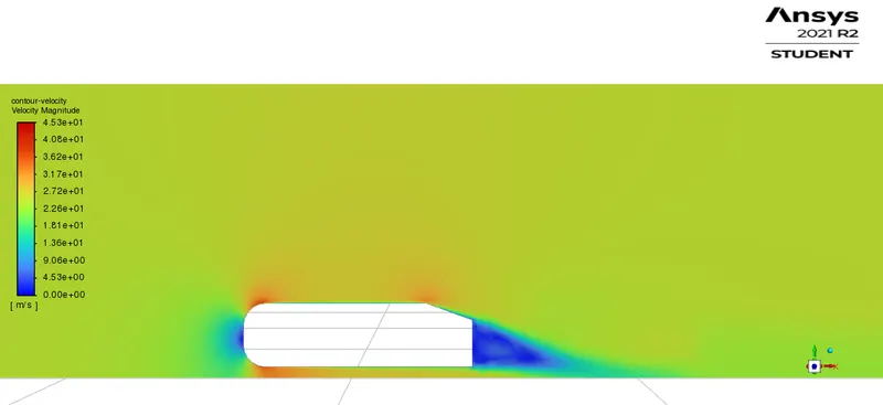
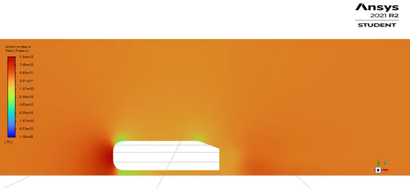
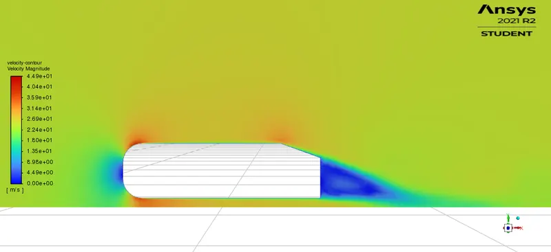
6. Velocity and pressure contours.
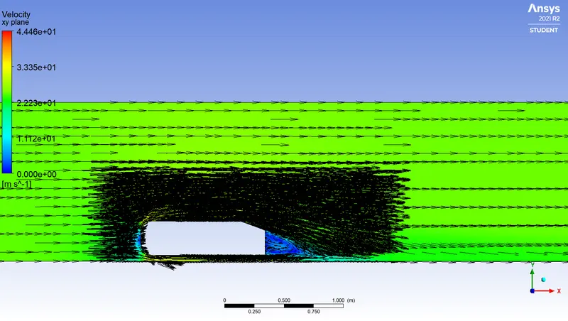
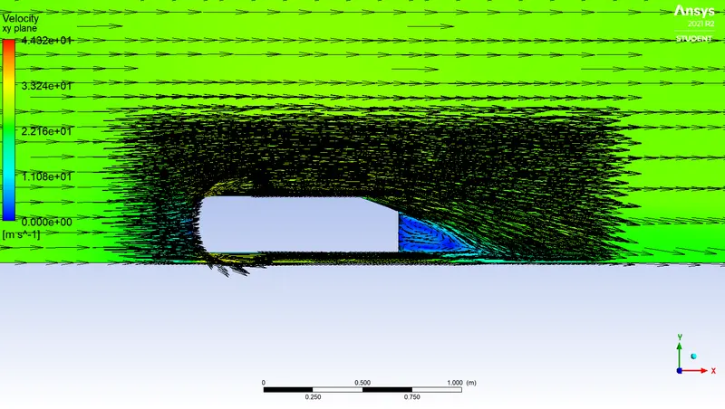
7. The vector plot clearly shows the wake region.

Methodology

• Introduction

1. Ahmed body and its importance

Ahmed body is a 3D model which is representative of a standard passenger car as shown in the diagram below. This is a research model proposed by S. R. Ahmed and Ramm while studying the geometry’s effect on the ground vehicle wake. The model is generally used to validate the CFD codes.

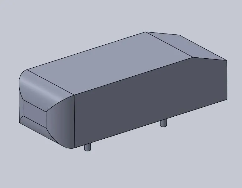
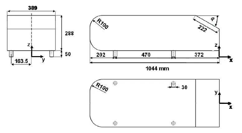
Since Ahmed body is a simplified car model, a lot of studies about the flow processes over this body have been conducted in order to understand the drag produced and other flow features like wake generation, separation, skin friction drag, etc. Since a lot of experimental data is available, it can be used to validate the numerical results of new car models.

Grid independency test

In order to study the flow properties on the Ahmed body, the model shown in the above figure has been chosen and velocity, pressure, drag plot calculated by following the following methodology in Ansys fluent. Different element sizes have been used by keeping the y+ = 200 near the wall to check the grid independence. First, we will start with the baseline meshing where we mesh the region around the Ahmed body with normal mesh generation.

Preprocessing

• Model creation (For Baseline Meshing)

We need flow around the Ahmed body and that is where the mesh needs to be created. There is no need to create mesh inside Ahmed body. Therefore a box covering the body need to be created.

A 3D model of Ahmed body has been imported into SpaceClaim and an enclosure of given dimensions is created.

For that, go to prepare tab click on the enclosure, uncheck the symmetric dimensions and enter the dimensions.

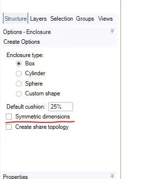
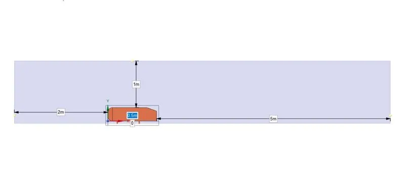
After entering the dimensions an enclosure is formed which encloses our Ahmed body ie, a volume subtracting the volume of Ahmed body.

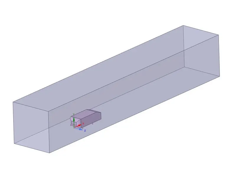
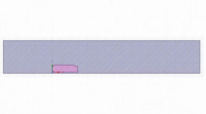
Since there is no need to generate mesh inside the body, suppress the Ahmed body for physics.

• Naming and meshing of the fluid domain

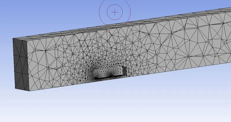
After creating the geometry file the next step is to divide the domain into small elements. Before that, we will assign names for different faces to apply boundary conditions easily. After that, the mesh has been generated by clicking on generate mesh.

• Setting up the problem

Here we set up the problem by applying relevant

1. Initial conditions
2. Boundary conditions
3. Material properties
4. Turbulence Models

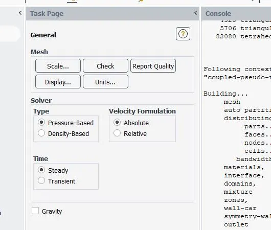
Here we are using a pressure-based (Mach number is less than 0.3) steady solver. The fluid is air with a freestream velocity of 25m/s.

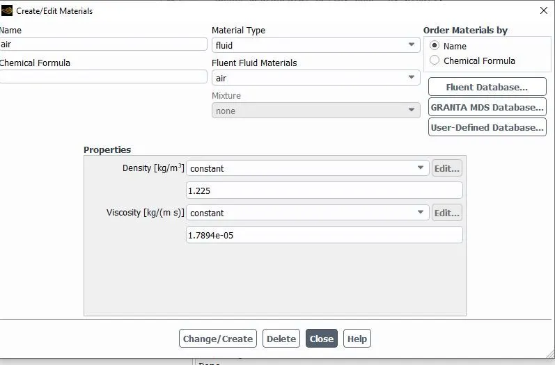
Material Properties

The fluid is Air, so the material properties of Air have been used.

Density =`1.225 (kg)/m^3`

Kinematic viscosity =`1.7894e-5 (kg)/(ms)`

Turbulence Model

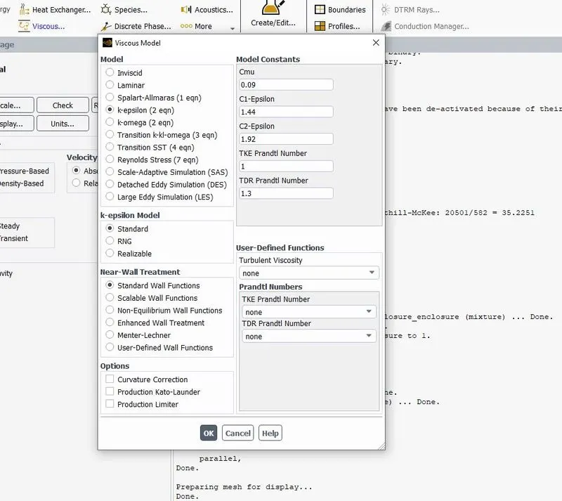
Reynolds number Re =`(ρuL)/μ = (1.225*25*1.044)/(1.7894e^-5)=1.787*10^6`

Since Reynolds number is greater than `10^5` the flow is turbulent. There we are using turbulence model as K-epsilon with standard wall functions.

Initial and boundary conditions

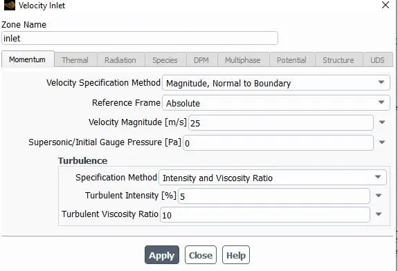
Inlet - Velocity boundary condition: Here the velocity magnitude is 25m/s

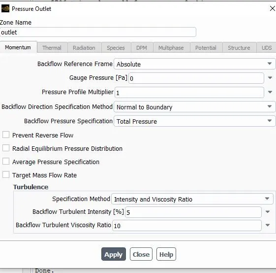
Outlet - Pressure outlet: Gauge pressure = 0

Car Wall – Wall: No-slip

Symmetry wall - Symmetry

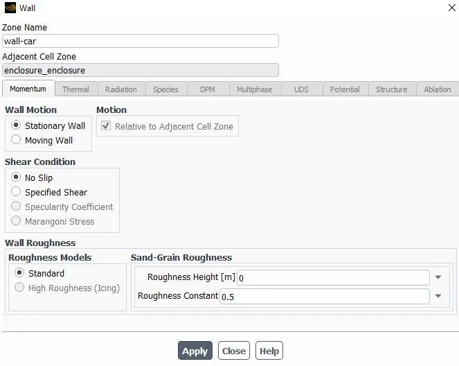
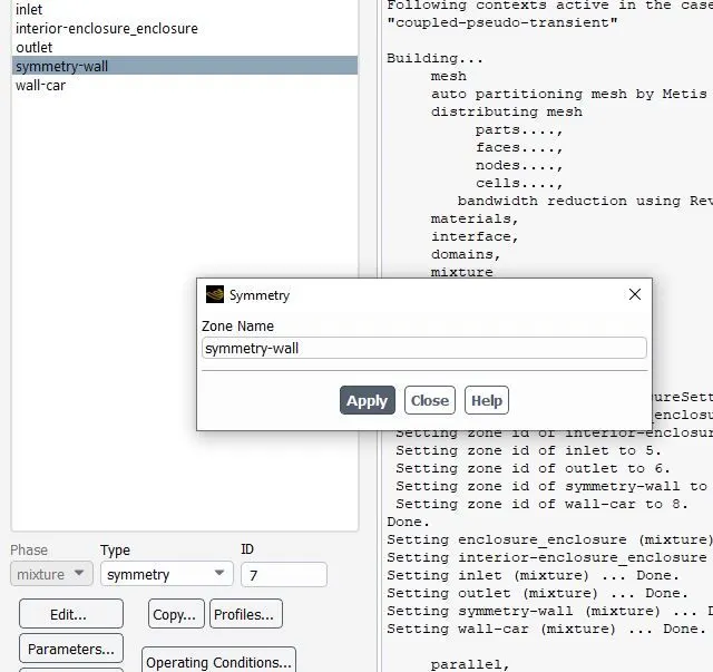
Reference Values

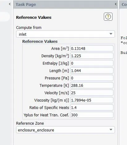
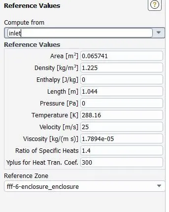
In order to get the correct drag coefficient, giving the correct reference values are very important. The following reference values have been used throughout the simulation.

Click on reference values under physics. Click on the inlet in the compute from the drop-down. Ensure that the area, density, velocity, and viscosity are as per our values. The area is nothing but the projected area.

Result extraction

Before running the simulation let’s set up some plots and curves for extracting results as the simulation proceed.

As we are interested in the physics around the Ahmed body, we will create a Section plane. Then, we will define pressure and velocity contours on that section place to visualize the pressure and velocity variations. To study the lift and drag coefficients on the body we will define lift and drag coefficient plots also.

Creating Monitor Plane

Go to results, click on create, then plane. Change the name as Cut plane z. Select XY plane as method. Put Z distance = 0.

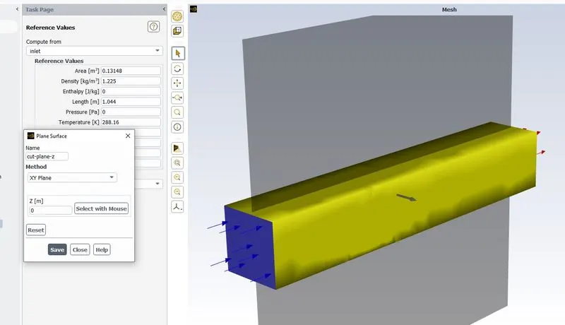
In order to see the Velocity and pressure contours are evolving while solving, we are creating contours before running the simulation.

For that first, we need to initialize the solution so that the solver gets the initial values of pressure and velocity. Later contours are defined from the results menu. The contour option will not be visible if the solution is not initialized.

After all the above steps let’s change the solution method to the standard scheme. Uncheck all the convergence in the residual menu since we want to see the solution till the completion of all the iterations. Then input the number of iteration=5 to start the simulation.

• Model creation (With local refinement)

In the above section, we created an unrefined mesh which resulted in much distorted results. In order to get a better result, we will add an additional area around the Ahmed body and make a more refined mesh.

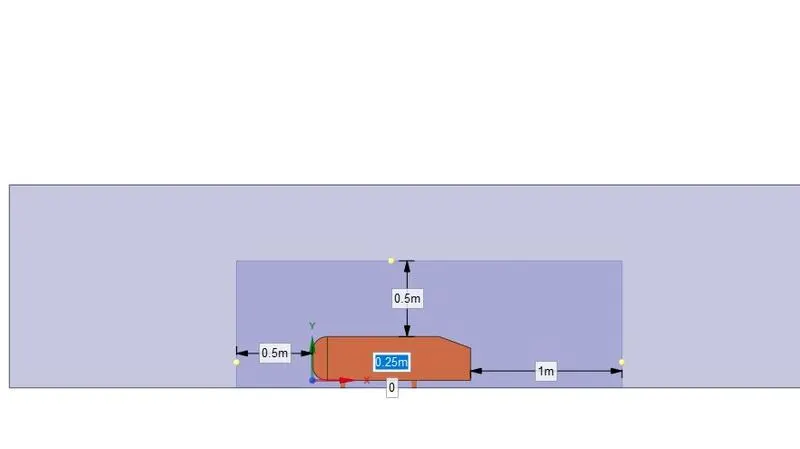
In Spaceclaim we will add another enclosure inside the main enclosure just above the Ahmed body. This is called local refinement.

As the body is perfectly symmetric, we can run the simulation by considering the only half body. By doing so, we can reduce the number of elements and get results faster.

For splitting the body, the split body option under the design tab is used in SpaceClaim. Using the split body option we select the body and then select the cutting plane. After that, we select the region to be removed. The outer enclosure is created as we did in the baseline model and the inner enclosure is also made. The dimensions of the inner enclosure are selected based on the wake region size that was seen in the baseline setup.

In order to avoid mesh overlapping, we need to remove the overlapping region of both enclosures by going into prepare, interference then clicking ok. This will solve the overlap problem. Once it is done we can see a clear cross-section of the geometry as below.

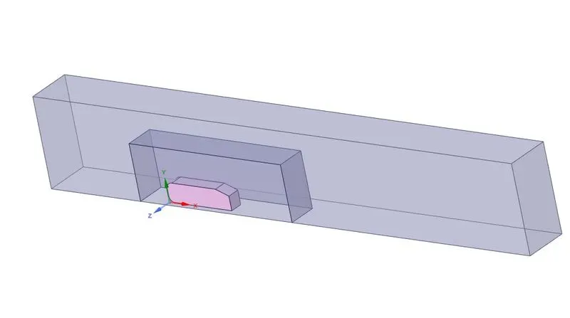
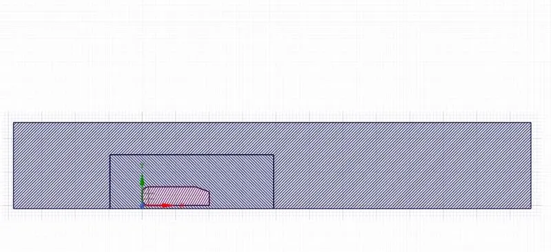
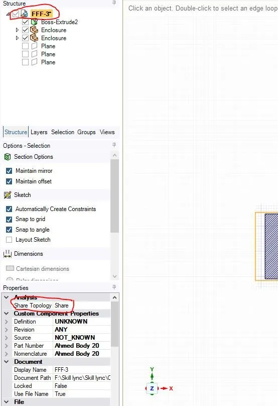
At last, ensure that share topology is set to share in order to make sure that the two boxes exchange information without any problems.

• Naming and meshing of the fluid domain

After naming all the faces and walls we will proceed to the meshing.

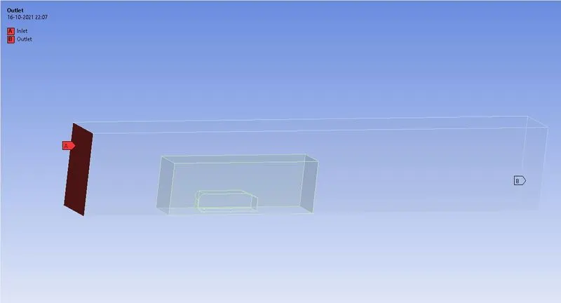
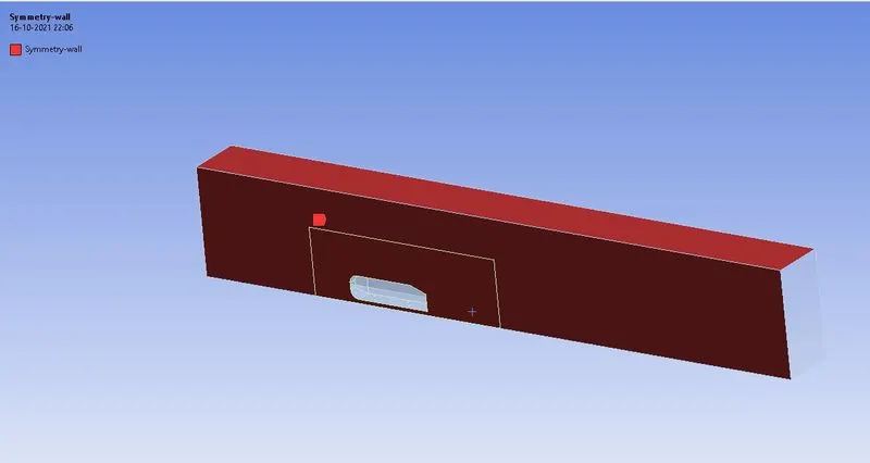
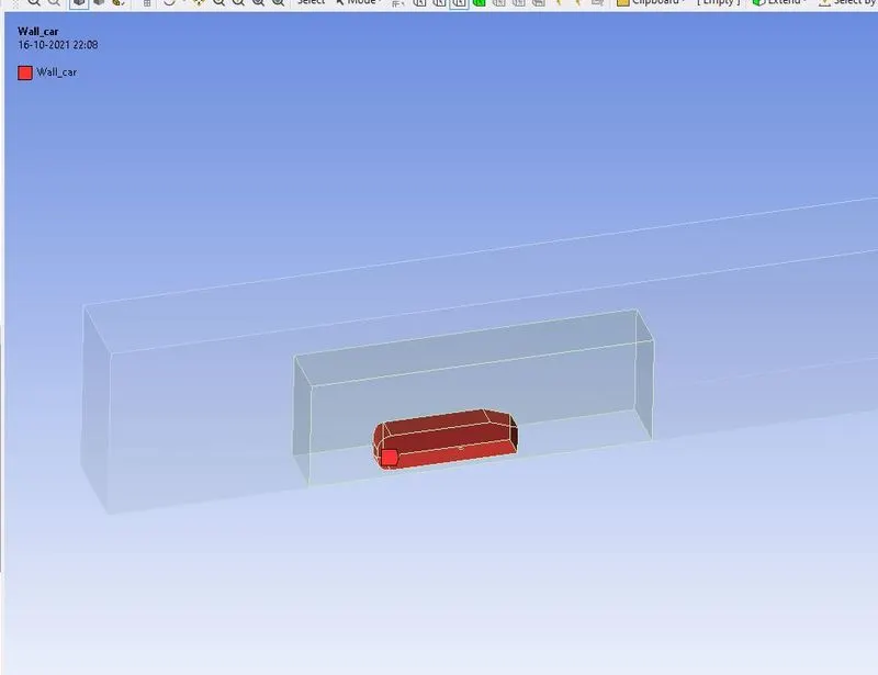
Outside the inner region, we have a perfect structure made up of straight lines without any complex shapes. Here we will use hexahedral meshes since it has the highest quality of all mesh types. For this, we have to create a method on the outer body.

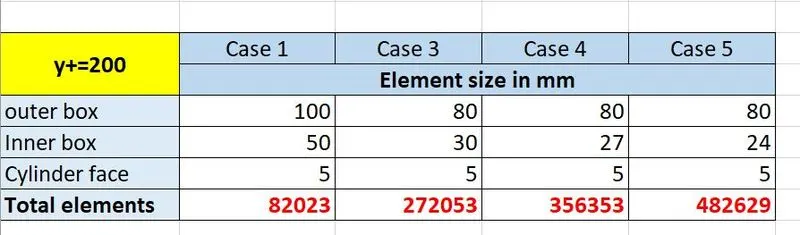
Right-click on mesh, go to insert then click on method. Under scope select the outer body as geometry. Change method to MultiZone. Under the mesh properties, change element size to 100 mm and maximum size to 100mm, then click on generate the mesh.

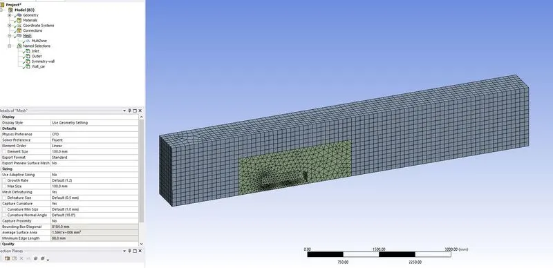
The next step is to refine the inner region. Right-click on mesh click on insert and navigate to sizing. Select the inner body as geometry and change the element size to 50 mm. Click on generate to update the mesh.

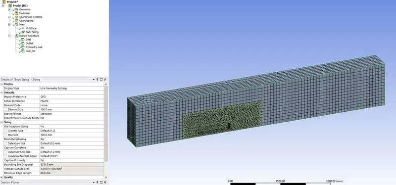
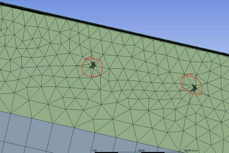
Now we can see a much more refined inner region. But if we check the cylindrical support region, we can see the faces are approximated as polygons. So, let’s do some refinements to make it circular. Right-click on mesh click on insert and navigate to sizing.

Select the 2 cylindrical faces as geometry, change element size to 5 mm. then click on generate the mesh. Now the cylindrical faces are refined better.

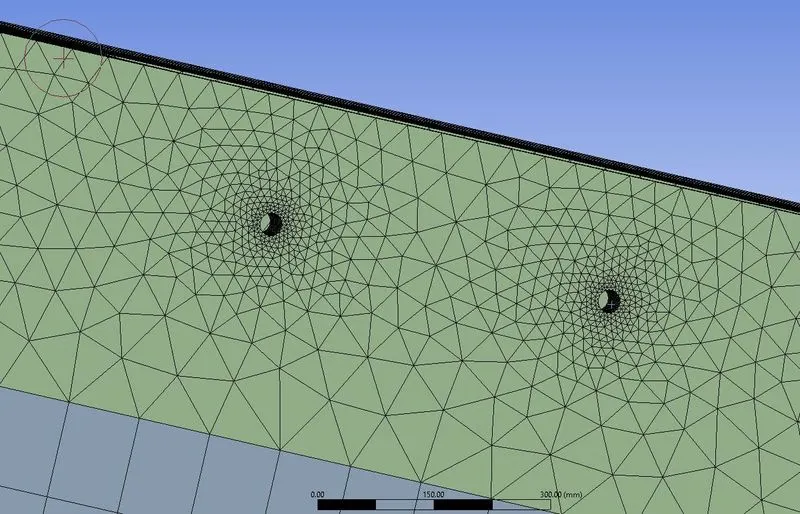
In order to capture the physics near the wall, we need to create inflation layers around the wall. Because, as the flow is turbulent there will be a small laminar region near the wall and if we are to resolve the gradients at such a small region we need a very small grid size.

Go to the properties of mesh, there we will see inflation, under inflation change use automatic inflation to All Faces in Chosen Named Selection. Select Wall_car. Change inflation options to total thickness. The number of layers = 6. The total thickness is calculated from the first layer thickness. The first layer thickness is calculated from the y+ value.

The equation for first layer thickness `y= (y^+ μ)/(ρu_t )`

Where, `u_t= √τ_w/ρ` = Frictional velocity

Here `u_t` can be calculated from wall shear stress `τ_w` which is again a function of skin friction drag coefficient `C_f`

`C_f=0.058Re^(-0.2)` For external flow.

`τ_w= 1/2 C_f ρU_∞^2`

If the `y^+` value is known, the first layer thickness can easily be calculated with the help of the above equations.

As for the problem, we will be maintaining `y^+` = 200.

Therefore from the above calculations, we can find that the first layer thickness y

`y=2.895 mm`

Total thickness for 6 layers = `28.7471 mm`

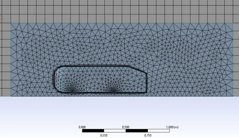
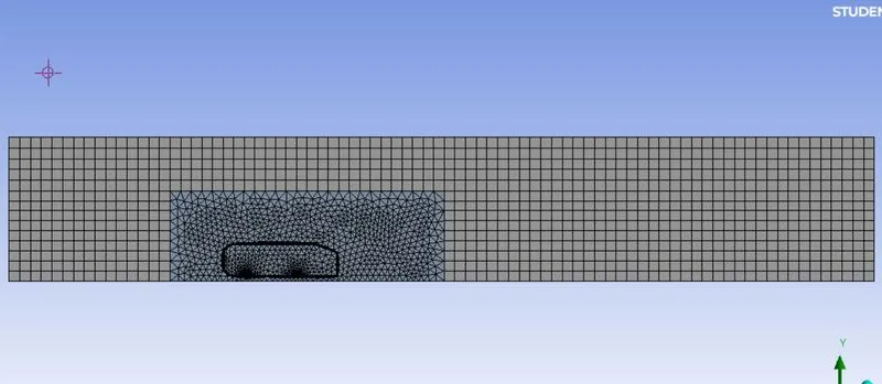
The above figure shows the mesh after taking a y+ value of 200. Throughout the problem, we will be considering y+=200 and for the grid independence test, different element sizes have been used in the outer box and inner box as per the below table

The solution setup is the same as the baseline setup except at the reference values. As we are using half the body the area in the reference values will change accordingly.

Postprocessing

• Solutions: Baseline meshing

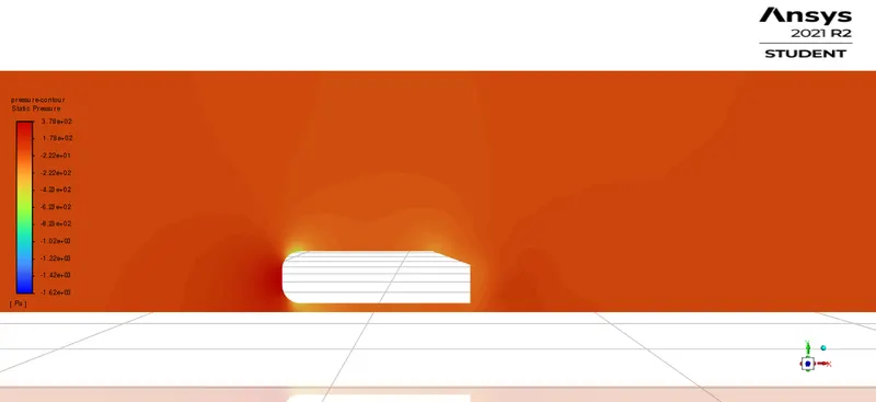
• Velocity and Pressure contours

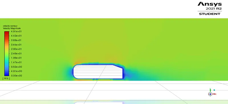
The above graph shows the velocity distribution. The flow is not clearly developed in this plot as the results are obtained from baseline meshing. This is reflected in cd, cl, and vector plots as well.

• Drag coefficient plot

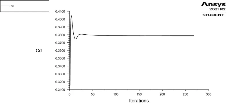
Coefficient of drag = 0.37891

• Lift coefficient plot

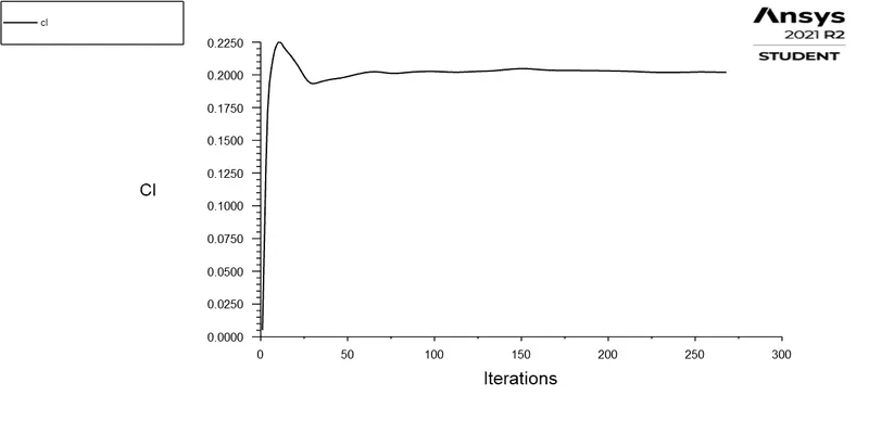
Coefficient of Lift = 0.20203062

• Vector plot

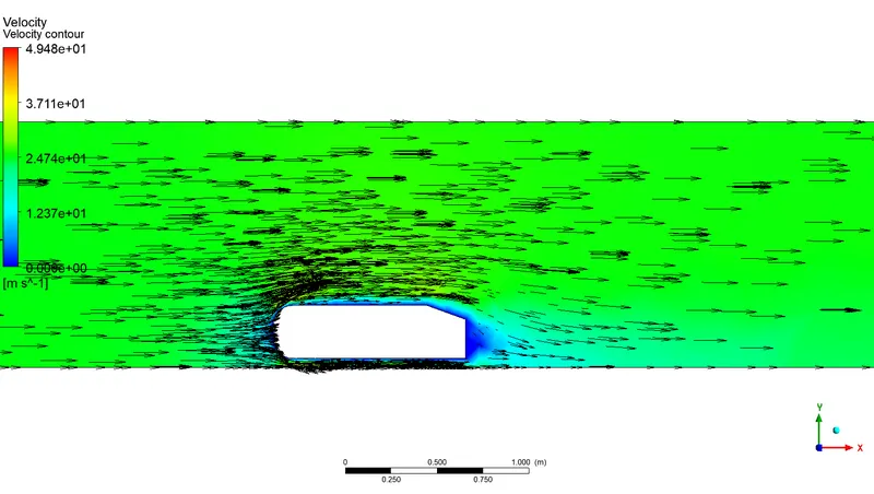
The wake region is not clear in this baseline meshing result.

• Solutions: Case 1: 82023 elements

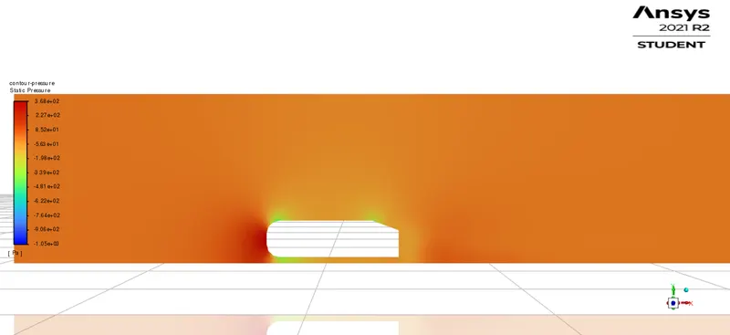
• Velocity and Pressure contours

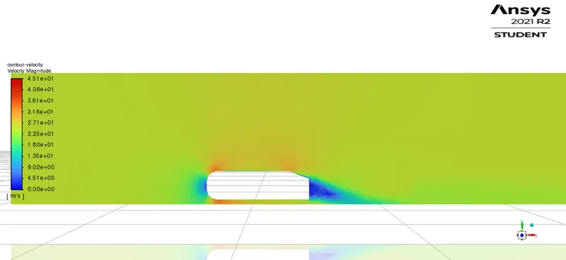
The above graph shows the velocity distribution. A clear flow region is started to visible by refining the mesh around the Ahmed body. This is reflected in cd, cl, and vector plots as well.

• Drag coefficient plot

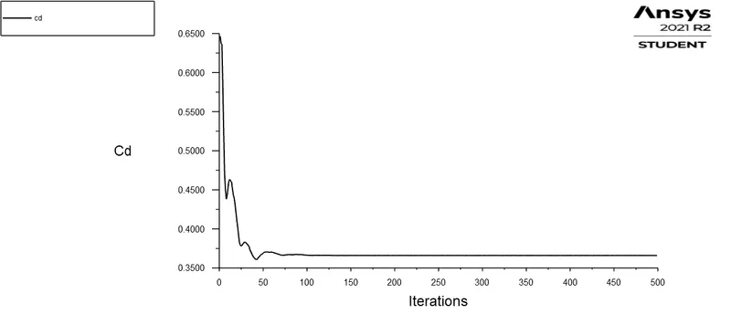
Coefficient of drag = 0.36596371

• Lift coefficient plot

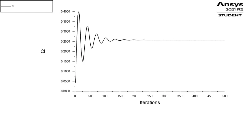
Coefficient of Lift = 0.25636184

• Vector plot

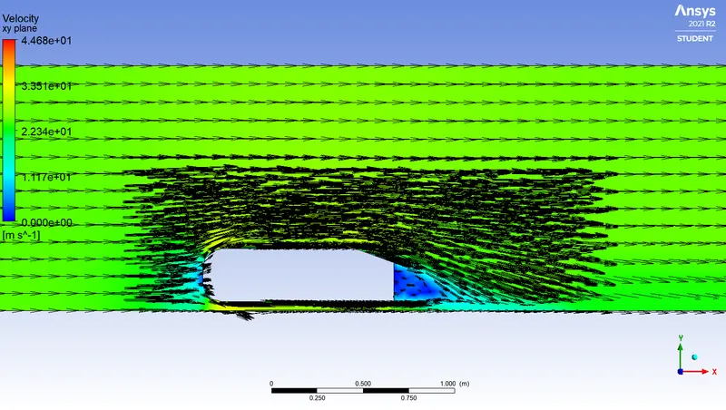
The wake region is visible in this refined meshing result with 82023 elements.

• Solutions: Case 2: 272053 elements

• Velocity and Pressure contours

• Drag coefficient plot

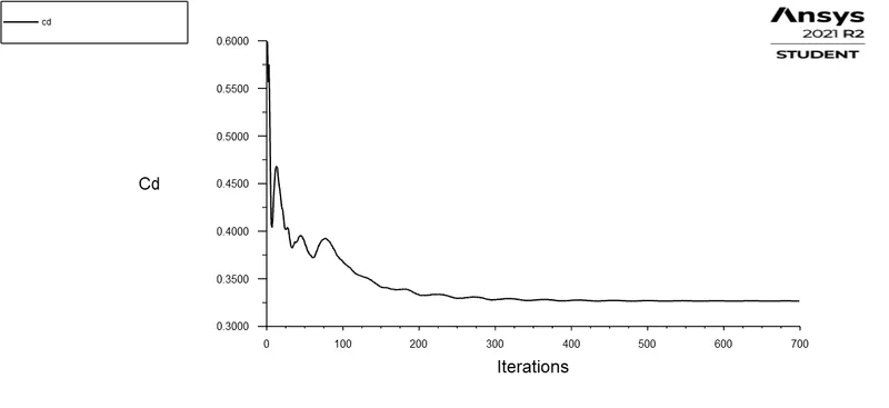
Coefficient of drag = 0.32665

• Lift coefficient plot

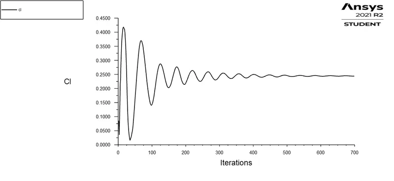
Coefficient of Lift = 0.24400991

• Vector plot

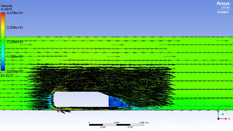
• Solutions: Case 3: 356353 elements

• Velocity and Pressure contours

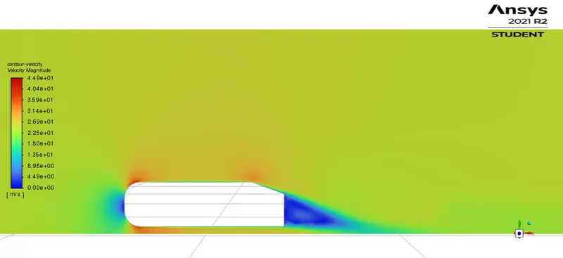
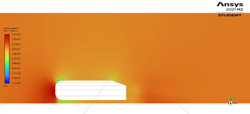
• Drag coefficient plot

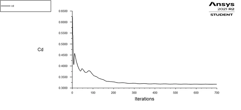
Coefficient of drag = 0.31731729

• Lift coefficient plot

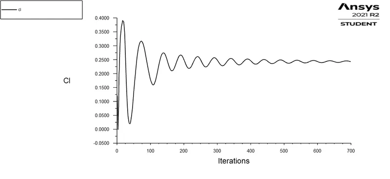
Coefficient of Lift = 0.24263209

• Vector plot

• Solutions: Case 4: 482629 elements

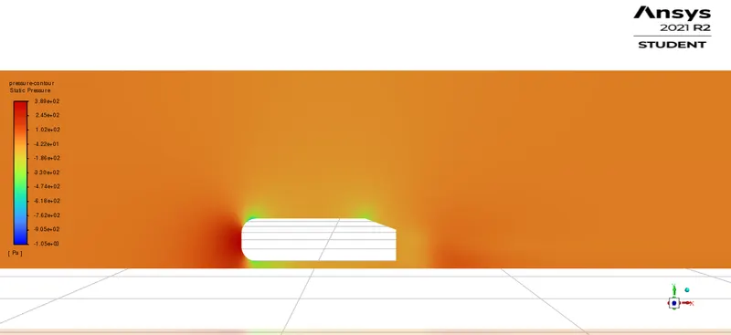
• Velocity and Pressure contours

• Drag coefficient plot

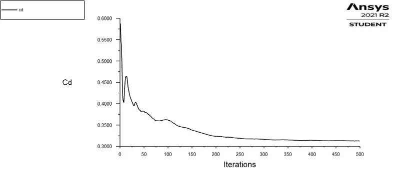
Coefficient of drag = 0.31302859

• Lift coefficient plot

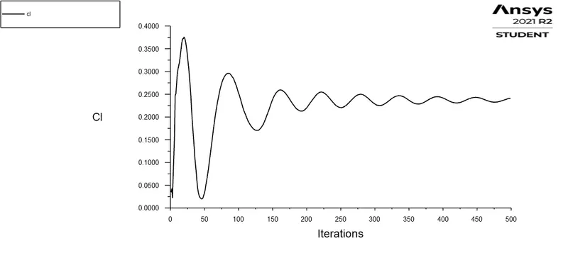
Coefficient of Lift = 0.24149453

• Vector plot

• Results and Discussion

From the data obtained from the simulations that we have conducted, we can segregate the data as in the below table.

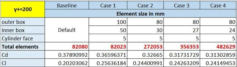
The following things were observed from the plots,

1. The baseline meshing results show inaccurate results with a marginal error in lift and drag coefficient. And, the wake regions are not prominent in this case.
2. Even in case 1 with refined mesh settings the results are not promising as the number of elements is not enough to capture the complete flow phenomena. Even though results are promising this refined mesh arrangement succeeded in capturing the wake region behind the Ahmed body.
3. In case 3, with higher refined mesh settings the results obtained are very close to the theoretical solution. Also, we can observe a developed flow over the Ahmed body.
4. As the refinement increases (from case 3), we can observe that there is not much change in the drag and lift coefficients. This tells us that grid independence has been achieved. Because there is not much difference in final results even if we increase the number of elements (from case 2).

• Negative pressure in the wake region.

As the flow hits the Ahmed body in the front, a stagnation point is created where the velocity is zero and the pressure is maximum. As the flow progresses along the body the velocity increases and a favorable pressure gradient (dp/dx<0) generates until it reaches the angular region of Ahmed body. As the flow reached the slant region it tries to follow the path. During this process, there would be an excessive momentum loss near the wall as the flow is trying to move downstream against increasing pressure inside the boundary layer (adverse pressure gradient dp/dx>0). If the adverse pressure gradient is dominating it would force the fluid particles inside the boundary layer. When this happens the particles are forced to move away from the body surfaces followed by creating a low pressure or wake region. This is also called separation. These pressure drops will create a high drag force against the flow.

• The significance of the point of separation.

The separation point is the point at which the flow detaches from the body. When the flow separates from the body it creates a wake region underneath which further increases the overall drag. In real life, one of the objectives of flow simulation over an Ahmed body or any object is to reduce the drag induced by the flow. It can be achieved by keeping the flow attached to the body as long as possible. In other words, delaying the point of separation. Hence Separation point is very significant.