Week 3 - External flow simulation over an Ahmed body.

Ahmed's body and its importance.

in 1984, S.R. Ahmed introduced a car lie geometry in his research called “Some Salient Features of the Time-Averaged Ground Vehicle Wake”. Later its known as Ahmed body. It has become a benchmark for aerodynamic simulation tools. The simple geometrical shape has a length of 1.044 meters, a height of 0.288 meters, and a width of 0.389 meters. It also has 0.5-meter cylindrical legs attached to the bottom of the body and the rear surface has a slant that falls off at 40 degrees. A large number of experimental data are available for this body so that it’s the best way to validate the simulation tools. The geometry of Ahmed body is shown below.

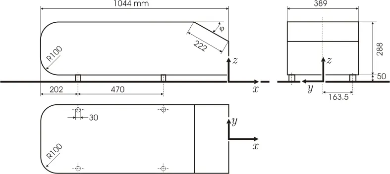
The Ahmed body helps us to capture the various aspects of airflow around the vehicle body, can be used to calculate the turbulence of flow around the car geometry and is used for studying various properties like drag coefficient, turbulence, lift forces etc.

Setting Up the simulation

Geometry

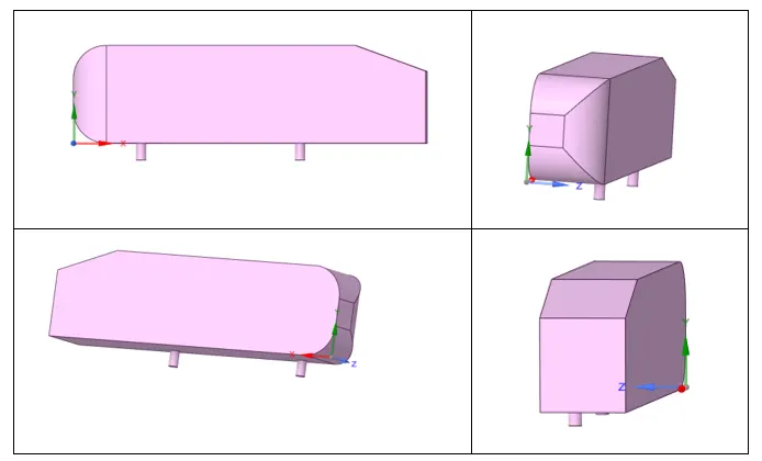
The generic Ahmed body geometry has been used for the simulation. Since the body is symmetric with respect to a plane only half of the model has to be solved computationally. Which will reduce the element size by 50 percentage. The geometry considered for the analysis is shown below.

Flow Domain

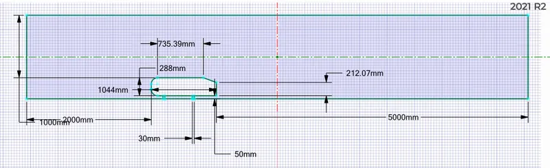
To Simulate the flow over an Ahmed body we have to construct an enclosure around the geometry and the image of the selected flow domain is given below.

Numerical discretization

After constructing the flow domain, it has to be discretized to small elements in order to implement FVM codes for that Meshing has been done. Here in total 4 different meshes are used.

During Meshing, we have to incorporate inflation layers to capture the physics more precisely. To calculate that one should be aware of the parameter called y+. Let’s go through that.

In turbulence modelling, the near-wall mesh size determination is very important in solving the turbulent models. But how small should be the mesh has to be kept for obtaining the exact turbulent modelling is a key idea. This is where the Y+ value comes into play, where it determines the first cell height from the wall. The Y+ plus value is dimensionless and is defined as the distance from the wall to the first cell. To understand the Y+ value let's first discuss boundary layer theory.

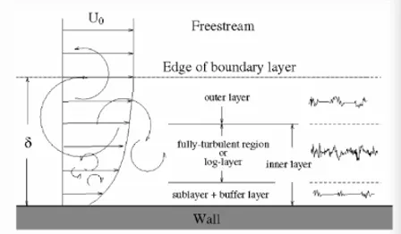
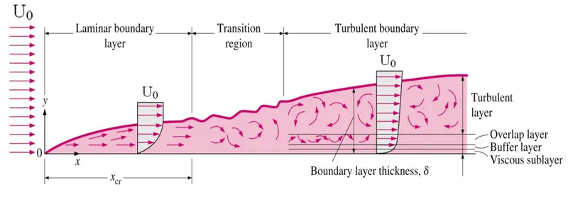
From the above figures, we could see that in the log layer the flow is fully turbulent. That Means, the velocity is very high leading to a higher Reynolds number. In this area, the inertia forces dominate the viscous forces. As we move closer to the wall where y value tends to zero the viscous forces dominate as we know that near-wall the flow velocity is zero. This region is called the Viscous sublayer. In the transition layer where the laminar flow transition to the turbulent flow neither of the law holds. In terms of y+value, we can say that

In viscous sublayer it is 1 <Y+<5

In the transition layer, it is 5<y+<30

In the log layer, it is 30<y+<500

From the above discussion, we can say that placing the first cell in the mesh region is very vital to determine the turbulent model and as well as to compensate for the computational mesh and time. The procedure for solving first cell thickness is given below.

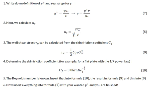
For the sake of accuracy, a MATLAB Program has been made to compute the first cell height.

% Matlab code for calculating first cell height for K-epsilon 

Y_plus = 3;
rho = 1.225; %Density in kg/m3
U = 25; %velocity in m/s
L = 1.044;  % Dia in meters
mu = 1.79*1e-5; %viscosity in Pa.S
Re = (rho*U*L)/mu ; %Reynolds Number
Cf = 0.058/(Re^0.2); %Coefficient of friction
Tw = 0.5*Cf*rho*(U^2);  %Wall shear stress
ut = (Tw/rho)^0.5; % friction velocity
First_Cell_Thickness = 2*((Y_plus*mu)/(ut*rho))*1000 %first cell height in mm

A Baseline mesh, a refined Mesh, and 3 more meshes with finer mesh size have been used for the study. The various indicators for all these cases have been summarized in the table below.

	Baseline mesh	Mesh with local sizing	Refined Mesh (10%)	Refined Mesh (20%)	Refined Mesh (30%)
Mesh (right click and Open image in new tab)
Element size	818.4 mm	100 mm	90 mm	80 mm	70mm
Body sizing	NA	30 mm	27 mm	24 mm	21 mm
Face Sizing	NA	10 mm	9 mm	8 mm	7 mm
Maximum Skewness	0.724	0.838			0.840
Number of elements	41649	434982			1290431
Total Thickness of inflation layers	2.7932	2.7932	2.7932	2.7932	2.7932
cd	0.399	0.287	0.278	0.283	0.286
cl	0.302	0.229	0.238	0.238	0.238

Mesh Independence test.

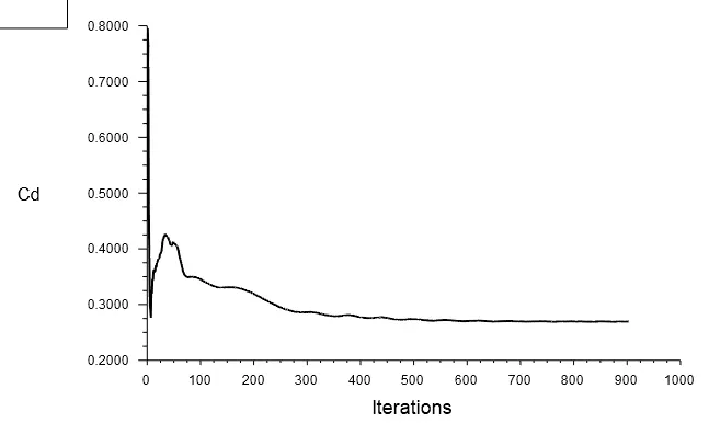
Apart from the Baseline mesh, 3 other meshes are used for the study. A target y+ value of 250 has been used for meshing. When the Mesh size was reduced by 20 percentage the change in the coefficient of drag and lift was changed by 7.19 and 21 percentage. Further reduction in mesh size by 25 percentage a change in the coefficient of drag and lift were changed by 1.292942 and 8.527891 percentages respectively. Further reduction in meshing will make the process too lengthy due to the high mesh count.

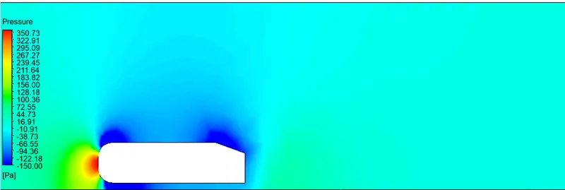
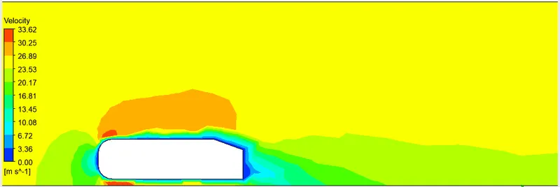
Mesh 1 : Base Line Mesh

Pressure contour

Velocity contour

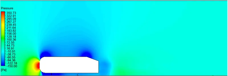
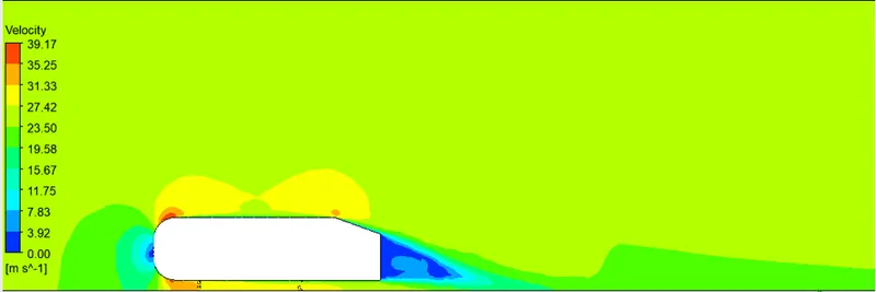
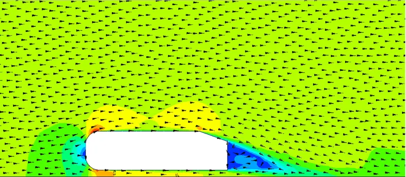
Mesh 2: Mesh with local sizing

Pressure contour

Velocity contour

Vector plot

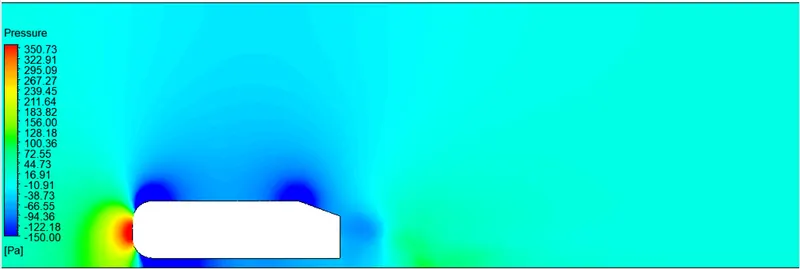
Mesh 3: Mesh with 10% refinement

Pressure contour

Velocity contour

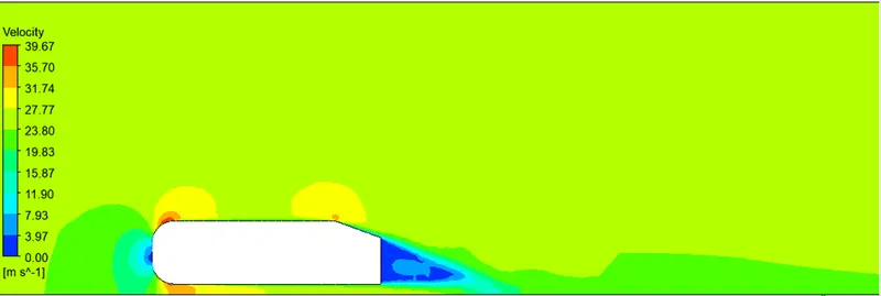
Vector plot

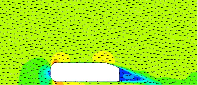
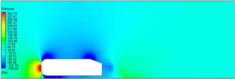
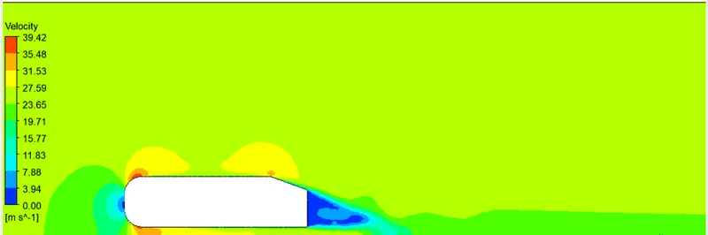
Mesh 4: Mesh with 20% refinement

Pressure contour

Velocity contour

Vector plot

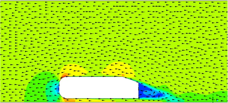
Mesh 5: Mesh with 30% refinement

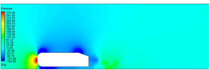
Pressure contour

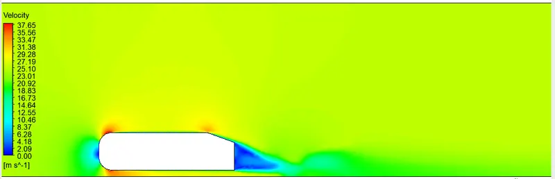
Velocity contour

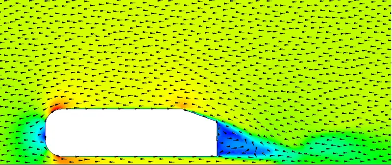
Vector plot

Plot for CD

Reason for negative pressure in the wake region:

The path lines showing the exact circular motion or vorticity generation just at the rear end of the car. The separation takes two regions of distribution. One at the upper part of the rear and the other at the lower part of the rear end.

The path lines show about the nature of the fluid interaction with the rear end of the Ahmed body which here shows that the fluid just after leaving the contact from the slope still possess the momentum in it and the fluid particles near to the surface almost show the no-slip region which means the very least possible velocity of the fluid particles is in contact with the slope and base of the rear part. Thus the fluid particles away from the rear region having the higher pressure beside the wake region try to approach from the higher pressure region to the lower pressure region thus creating a circularity exactly in the wake region created.

The body penetrating the fluid creates a region of emptiness just beside its end due to the nature of the geometry of the body here which can be seen least in case of a perfectly streamlined shaped body. This emptiness created is a low-pressure region towards which the fluid column exactly behind the wake region which of atmospheric pressure tries to fill the space thus dragging the fluid column with it thus creating the region of vorticity. This also results in the huge pressure gradient in the region exactly rear of the body creating the –ve pressure at the end. Also, this is the layman’s reason why there is negative gauge pressure in the wake region.

Significance of the point of separation

The fluid separation point can be defined as a point where the dv/dy i.e. gradient of velocity goes zero along with the dp/dx = 0, for the specific point. In more simplified term we can say that the point where the velocity gradient goes zero and the pressure gradient along the x- direction goes zero the point of separations starts occurring or the negative pressure gradient starts forming after that point. The point of separation cannot be understood just by single contour in hard and fast way. It can be supportively studied with the help of the dp/dx plots or velocity plots w.r.t the Y direction and other such plots in which we can see the nature of such physical properties like dp/dx=0, and dv/dy=0 experiencing in a particular region of fluid and body interaction.

CONCLUSION

• We can use a sectional part of the geometry if the geometry is symmetrical it helps in increasing mesh grid element cells also leads in reducing the computational time.
• We can verify the results got from the simulation to validate our simulation setup for actual geometries of Ahmed body.
• Using Y+ value to generating mesh improves the accuracy at the car-wall surface when the flow is turbulent, it also affects the accuracy of drag and lift coefficients.
• A grid independence test is important to validate the generated mesh of the final setup as it stablises the resuls.
• A hight turbulent zone is created at the wake zone & there is negative pressure created due to boundary layer separation.
• The boundary separation and recirculating of the flow and also the effect of shear stress. To overcome the shear, stress pressure turns negative to balance the effect.