Week 3 - External flow simulation over an Ahmed body.

AIM:

To study the aerodynamics of the Ahmed's body by running the simulation for the velocity of 25m/sec with the default air properties in Fluent.

OBJECTIVE:

1. To describe Ahmed's body and its importance.
2. To explain the reason for the negative pressure in the wake region.
3. To explain the significance of the point of separation.

EXPECTED RESULTS:

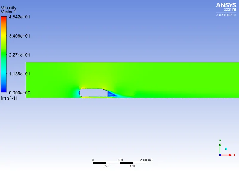
1. Velocity and pressure contours.

2. The drag coefficient plot for a refined case. ( For velocity of 25m/sec, the drag coefficient should be around 0.33).

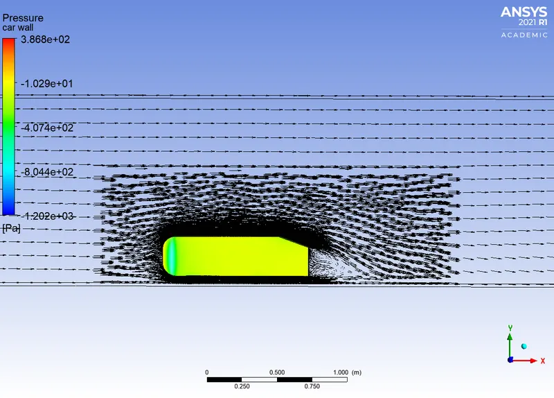
3. The vector plot clearly showing the wake region.

4. Perform the grid independency test and provide the values of drag and lift with each case.

INTRODUCTION:

Optimized external car aerodynamics is necessary to achieve efficient vehicles with minimized fuel consumption, `CO_2` emissions, and noise, while keeping a good driving stability. Steadily increasing computer power has been raising the importance of simulating the external aerodynamics of vehicles and computing the corresponding aerodynamic characteristic numbers. At present, an efficient resource management gains increased importance everywhere. A substantial part of the development time of cars is therefore invested in optimization. This is possible only and particularly by virtual development. In order to establish such development processes in the car industry, reliable simulation models validated by experiments are needed.

Model experiments suitable for providing validation data make use of model bodies with geometries characterized by variable parameters, such as the slant angle at the back. One such body is the Ahmed body, a bluff model body of simple shape with basic aerodynamic properties of a vehicle, which has been used for many reference investigations.

THEORY:

Ahmed's Body and its importance:

• The Ahmed body represents a simplified, ground vehicle geometry of a bluff body type. It is a generic car body(a simplified car model) and its shape is simple enough to allow for accurate flow simulation but retains some important practical features relevant to automobile bodies. This model describes how to calculate the turbulent flow field around a simple car-like geometry.
• The air flow around the Ahmed body captures the essential flow features around an automobile and was defined and characterized in the experimental work of Ahmed. Although it has a very simple shape, the Ahmed body allows us to capture characteristic features that are relevant to bodies in the automobile industry.
• This model is also used to describe the turbulent flow field around a car-like geometry. Once the numerical model is validated with the experimental data from the wind tunnel test, it is used to design new models of the car.

The Ahmed body was described originally by S. R. Ahmed in 1984. Three main features were seen in the wake:

• The A-recirculation region that is formed as the flow separates at the top of the vertical back surface of the model.
• The B-recirculation region that is formed due to the separation at the base of the model.
• The C-pillar vortices that form as the vorticity in the side boundary layers roll up over the slant edges.
• The wake was shown to be highly dependent on slant angle. For slant angles less than 12°, the flow remains attached over the slant. The flow is essentially two-dimensional and has low drag. Between 12° and 30° the flow becomes much more three-dimensional as the c-pillar vortices form. These reach maximum strength at 30°. The drag increases significantly as the low pressure cores act on the rear surfaces. Past 30° the flow separates fully off the slant. This results in a sudden decrease in drag and weaker c-pillar vortices.
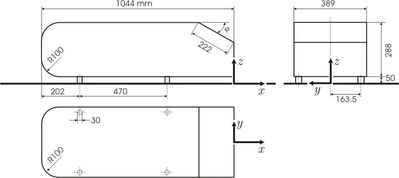
• The Geometry of Ahmed's Body is as shown in the below figure.

Aerodynamics of a Car body:

• The drag coefficient quantifies the resistance of an object in a fluid environment. It is not an absolute constant for a body's shape because it varies with the speed, direction of flow, object shape and size, and the density & viscosity of the fluid. The lower the drag coefficient of an object, the less aerodynamic or hydrodynamic drag occurs. In terms of a car, the lower the drag coefficient, the more efficient the car is. As well as affecting the top speed of a vehicle, the drag coefficient also affects the handling. Cars with a low drag coefficient are sought after, but decreasing the drag drastically can reduce the downforce and lead to loss in road traction and a higher chance of car accidents.
• There are certian ways to modify a car to optimize its aerodynamics and decrease the drag coefficient. To streamline the exterior, you can remove certain aftermarket items such as the roof rack, mud flaps, spoilers, and radio antenna. Professional car racers also take off their windshield wipers and side mirrors for better aerodynamic performance.
• For an ordinary car, it is recommended to add wheel covers, a partial grill block, an under tray, fender skirts and a modified front bumper to improve the drag coefficient and make the car stand out in the process.

PROCEDURE:

GEOMETRY:-

• First of all, we need to load the geometry of Ahmed's body in the ANSYS SpaceClaim.

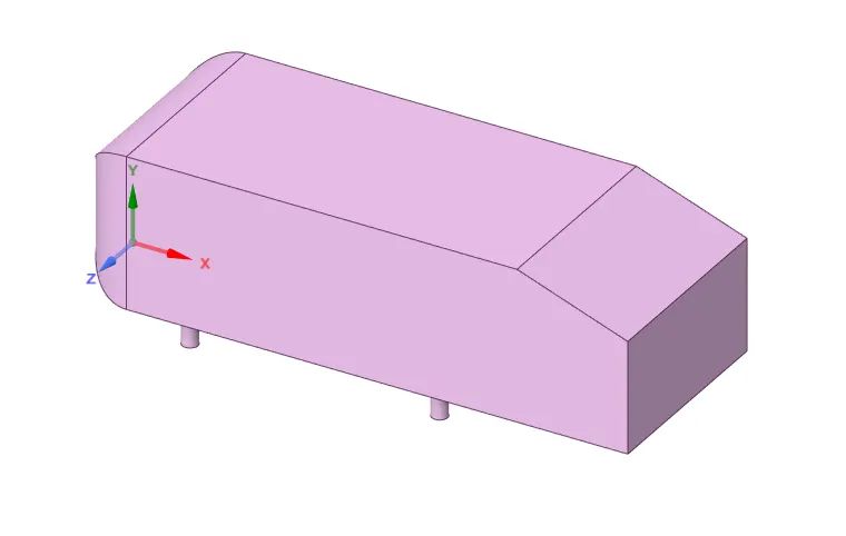
isometric view of the model

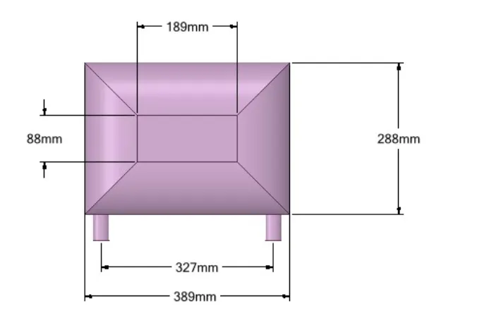
Front view of the model

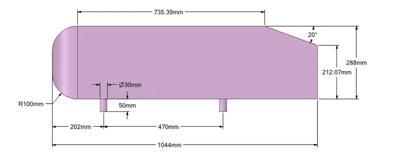
Side view of the model

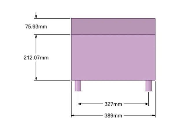
Rear view of the model

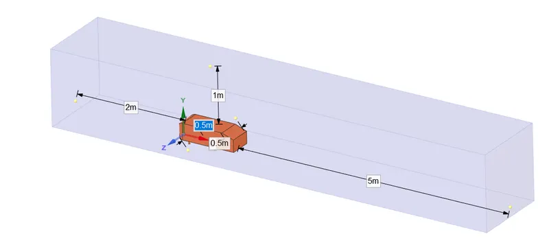
• Creating the outer enclosure as given below;

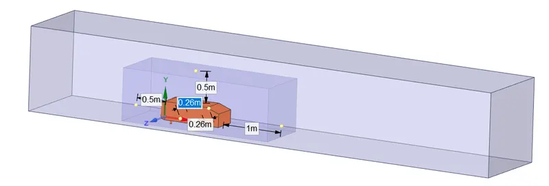
• Creating the inner enclosure as given below;

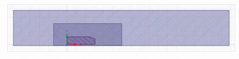
Sectional view

• From the above sectional view, we can see that the section of the two enclosures are interfering and hence, the meshing will be overlapped between the two enclosures.
• Using the 'interference' command, we can solve this overlapping by separating the two enclosures. Before that we have to check for share topology option to share.
• The ahmed body has to be suppressed using 'suppress for physics' option.

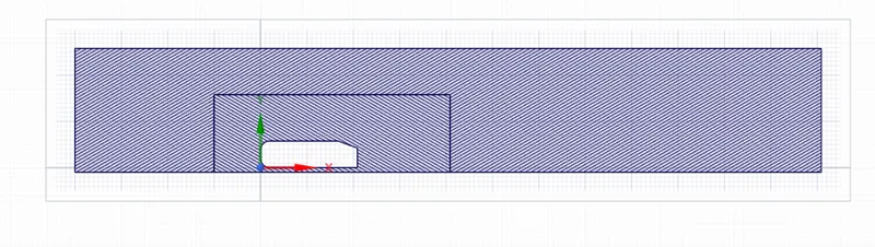
• As the body is perfectly symmetric, we can run the simulation by considering the only half body. This is the best practice where we can save on the number of cells and get the results faster as well.
• We can use the 'split body' command in Spaceclaim to perform the operation and then we can use the symmetry boundary condition in fluent to perform the simulation.

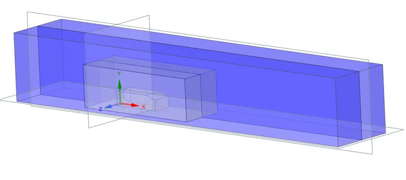
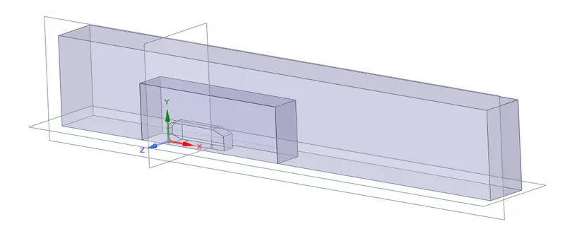
• Here, we have splitted the body into two halves and deleted or suppressed the one part for physics.

MESHING:-

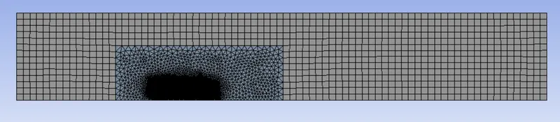
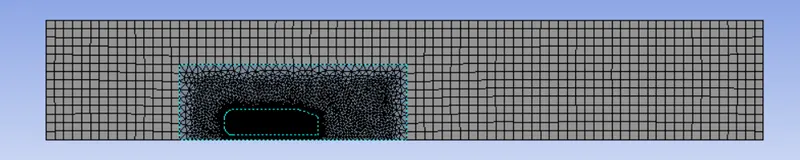
• Generating the mesh on the enclosures around the Ahmed body, the outer enclosure has been set as Hexahedral grids using 'Method--> Multizone'
• Assigning the boundary names for front side of the ahmed body as inlet, rear side as outlet, the top,bottom,left and right sides as symmetry and Ahmed body as car-wall.
• The outer enclosure has to be coarsened using 'Body sizing' option because there is not much of the flow going to be. The inner enclosue has to be meshed finer with face meshing.
• The Ahmed body has to be meshed finer than the inner enclosure to capture the flow accurately.

Importance of Y+

• The behaviour of the flow near the wall is a complicated phenomenon and to distinguish the different regions near the wall , the concept of `y^+` has been formulated. Thus `y^+`is a dimensionless quantity, and is distance from the wall measured in terms of viscous lengths.

• The y+ value denotes wherein the y+ vs u+ curve we are with respect to the cell size. It is undesirable to have a cell size that leads to a y+ of between 10 to 30 since the modeling of flows transitioning from laminar to turbulent is not easy and is still being researched.
• Due to this fact, it is better to have a y+ of less than 10 meaning we'd be at the laminar region or have a y+ of greater than 30 where we can go with a wall function and still achieve results.
• The y+ value can be used as a marker based on which we can decide on the base grid size and make a decision based on the computing power as to whether the grid needs to be refined further or coarsened.

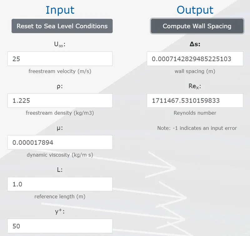
• Calculated the Y value or wall spacing by using the `y^+` calculator.

• we can also use empirial formulae to calculate skin friction coefficient `C_f` which are given as;

For internal flows -
For external flows -

• After calculating `C_f`, we have to calculate wall shear stress `tau_w`

`tau_w=(1/2)*C_f*rho*u^2`

• Then calculate the frictional velocity, `u_tau=sqrt(tau_w/rho)`
• Finally, substitute the values in the `y^+` formula to calculate the first grid point from the wall , `y^+=(y*u_tau*rho)/mu`
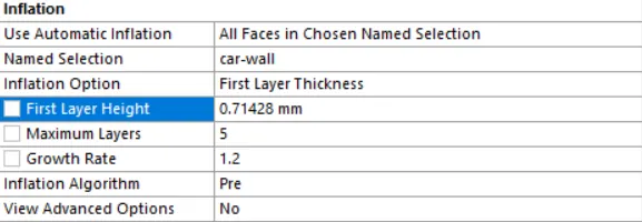
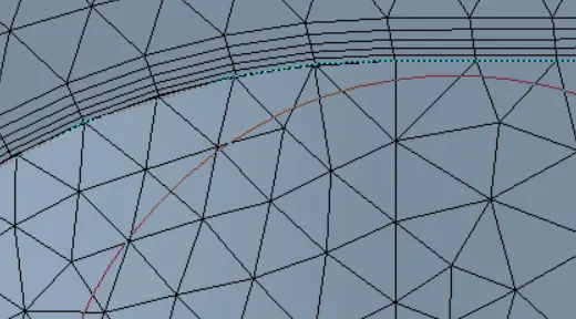
• Here, we have used 'inflation' layer to set-up the `y^+` value.

Element Quality

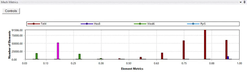
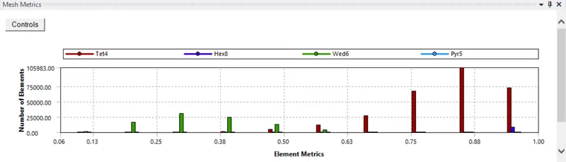
• Here, most of the elements fall above the 50% of Element metrics quality. So, it is a fine mesh.

FLUENT SET-UP:-

Pressure based solver vs Density based solver:

The pressure based solver traditionally has been used for incompressible and mildly compessible flows. The density based approach on the other hand was originally designed for high- speed compressible flows. Both approaches are now applicable to a broad range of flows (from compressible to highly compressible), but the origins of the density based formulation may give it an accuracy (i.e. shock resolution)capture advantage over the pressure based solver for high-speed compressed flows.

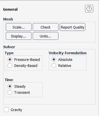
• In the setup, set Physics-->Solver type-->Pressure based solver. Since, the mach number of the flow is less than 0.3, it is an incompressible flow we will be using the pressure based solver.

• Check the energy , since we are going to deal with the temperature here.
• In the viscous model, go on with standard `k-epsilon` model because our flow is fully turbulent and set near wall treatment as 'standard wall functions'.
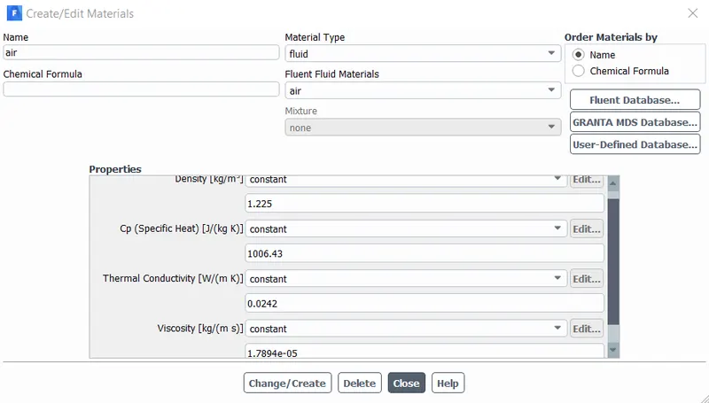
• The simulation has to be run with default air properties in fluent.

• setup>physics>Boundaries>inlet - velocity as 25m/s, outlet gauge pressure as 0 Pa and leave it the other conditions as the default values.
• setup>solution>solution methods>SIMPLE scheme for pressure-velocity coupling, since it is a pressure based solver.
• Whereas Coupled scheme will work good as well, it is a full implicit scheme and the momentum and continuity equations were solved simultaneously so, it will take more memory space and less time for convergence.
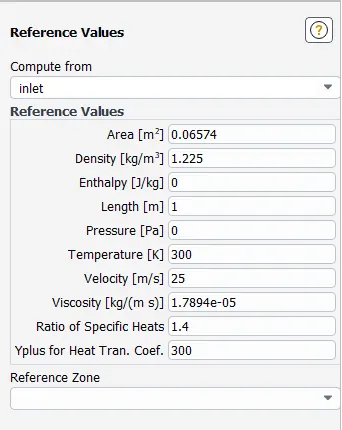
• setup the reference values for calculating the drag coefficient

• setup>solution>Report definitions>New>force report>drag>drag coefficient>car-wall>select report file and report plot>save/display and also same as that for Lift coefficient.
• setup>solution>Initialization>method>Hybrid>Initialize
• Results>create>Plane>point and normal and create a cut plane-z at a distance of 1m.
• setup>solution>Run calculation for 400 iterations.
• create contour plots for velocity and pressure from the results>graphics>contours>New for the cut plane-z.

CFD-POST:-

• In the CFD post, we can get the vector plots for velocity variable, velocity and pressure contour planes.

RESULTS:

Case 1:-

In the first case, the simulation was done with the following cell count;

• Y-plus = 50
• Viscous model: K-`epsilon`
• outer enclosure: 100 mm size of Hexahedral mesh
• inner enclosure: 50 mm size of tetrahedral mesh
• car body: 10 mm size of tetrahedral mesh
• inflation first layer thickness: 0.71428 mm
• No. of Elements: 329976
• Nodes: 99226

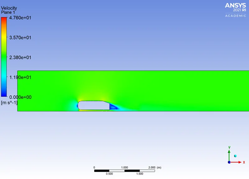
Velocity Contour plane

Pressure contour plane

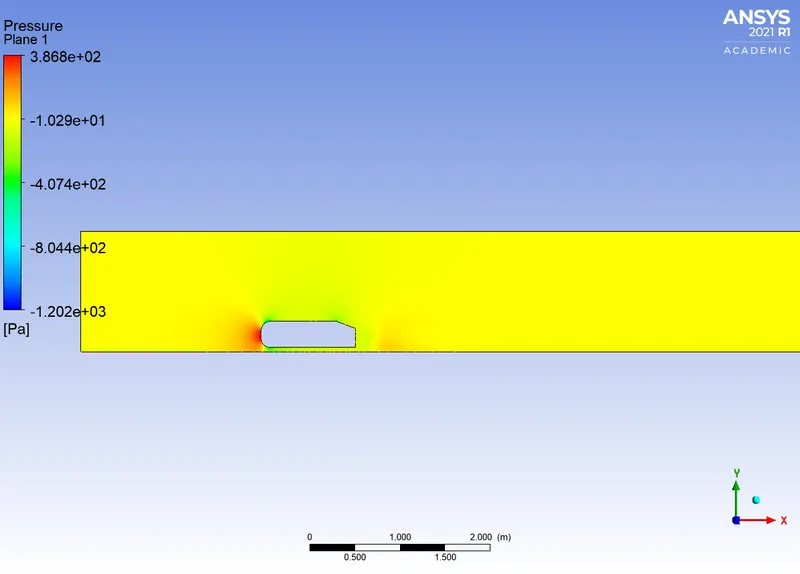
Reason for the negative pressure in the wake region:

• Wake is the region of recirculating flow immediately behind a moving or stationary blunt body caused by viscosity which may be accompanied by flow separation.
• The negative pressure is due to the velocity difference applied at a certain Reynold's number and the rear angle, which at a low Reynolds number when this difference in pressure happens the wake obtained increases the drag due to the pressure drop behind the Ahmed body, which at a high Reynolds number due to the vortices generated it produces small amounts of pressure thrusting the body.
• The air becomes almost stagnant as it strikes Ahmed body which results in air exerting very high pressure on the front face of Ahmed body. The airflow then gets divided between the upper and lower surface of the Ahmed body. The higher pressure air on the front surface accelerates as it travels over the curved nose surface of Ahmed body, causing the pressure to drop.
• This lower pressure creates lifts over the roof surface as the air passes over it. As the air continues to flow and make its way to the rear, a notch is created by the rear slant angle of 20 degree owing to flow separation, leaving a vacuum or low-pressure space which the air is not able to fill properly. The resulting lower pressure creates lift and the drag that then acts upon the surface area of the rear slant.
• The following figure shows the pressure thrusting.

Scaled Residuals plot

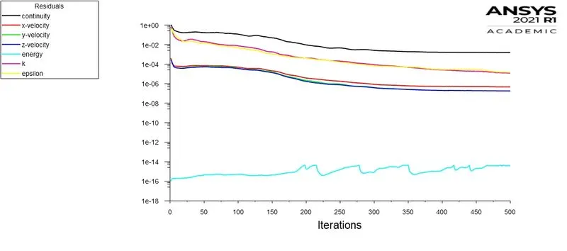
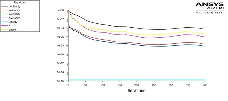
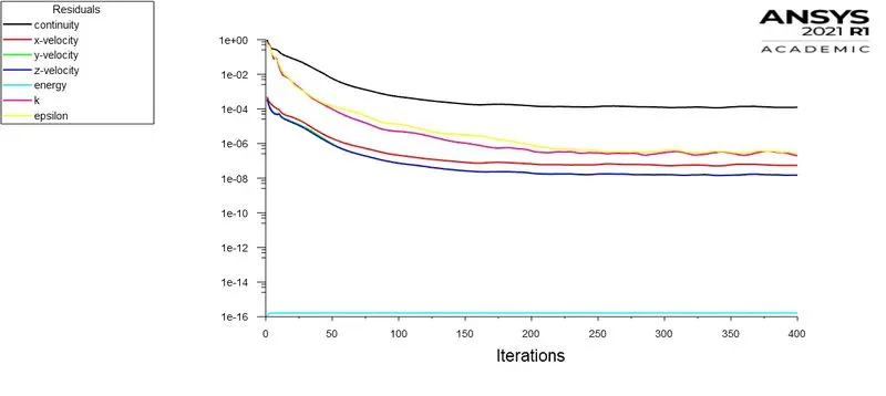
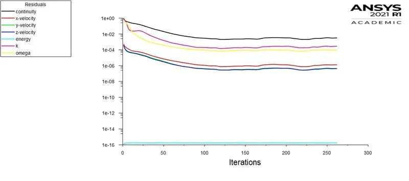
• Here, we can see that around 100-150 iterations the solution tends to converge.

Drag coefficient plot

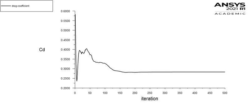
Lift coefficient plot

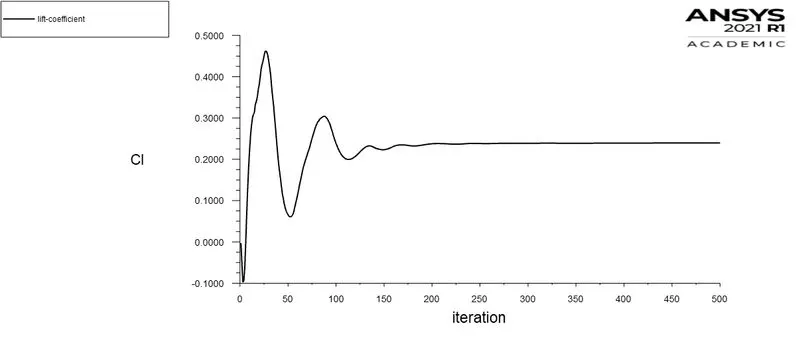
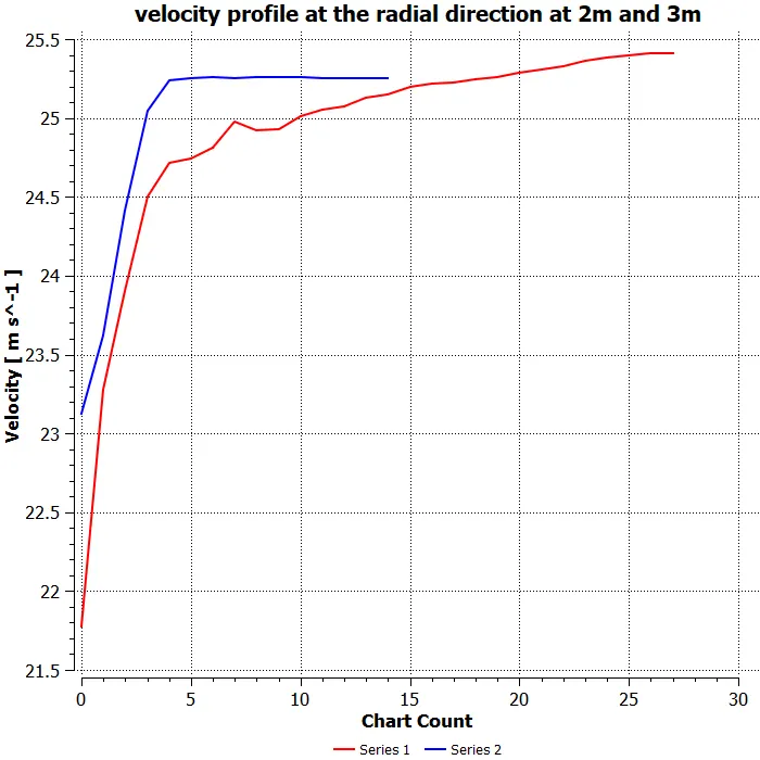
Velocity profile in Radial distance at 2m and 3m

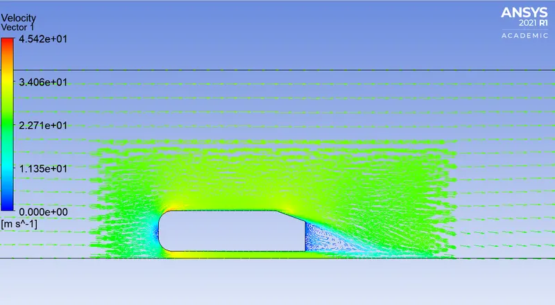
Vector plot clearly showing the wake region

Significance of the point of separation:

• Flow separation or Boundary layer separation is the detachment of a boundary layer from a surface into a wake.
• Separation occurs in flow that is slowing down, with pressure increasing, after passing the thickest part of a streamline body or passing through a widening passage.
• Boundary layer separation occurs due to the adverse pressure gradient which means the flow takes place from low pressure area to high pressure area.
• The point of separation defined by the Ahmed body and the flow, the alpha angle depending on which value is at it causes a change in the flow direction, forces required, lift on the body, induced drag due to 'tip vortex', at a critical value flow in slant stalls and reduced lift-reducing the drag as well, all depending on the value of alpha and the Reynold's number of the flow.

Case 2:- (Refined Case)

In the second case, the simulation was done with the following cell count;

• Y-plus = 100
• Viscous model: K-`epsilon`
• outer enclosure: 100 mm size of Hexahedral mesh
• inner enclosure: 35 mm size of tetrahedral mesh
• car body: 10 mm size of tetrahedral mesh
• inflation first layer thickness: 1.428 mm
• No. of Elements: 384578
• Nodes: 108773

Mesh size

Element Quality

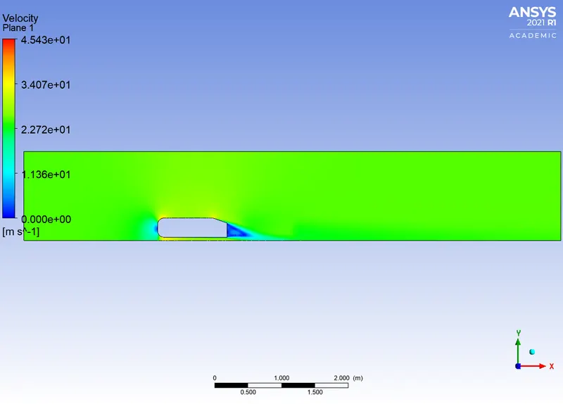
Velocity Contour plane

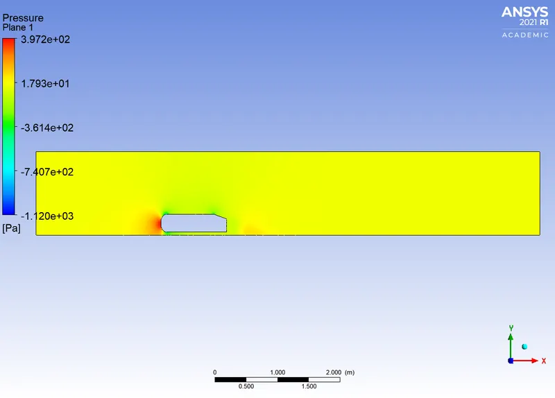
Pressure contour plane

Scaled Residuals plot

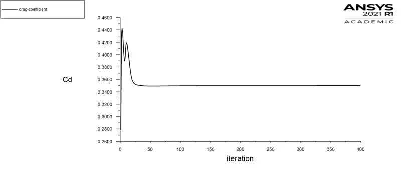
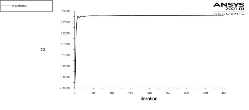
Drag coefficient plot

Lift coefficient plot

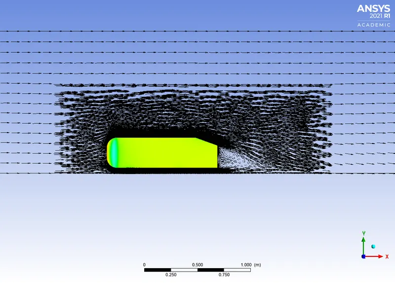
Vector plot clearly showing the wake region

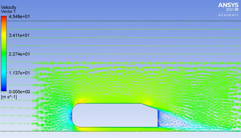
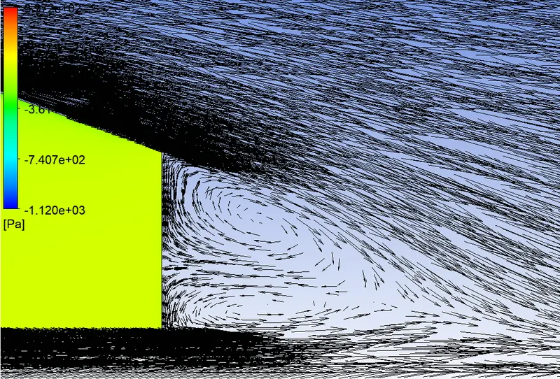
Recirculation region

Case 3:-

In the third case, the simulation was done with the following cell count;

• Y-plus = 125
• Viscous model: K-`epsilon`
• outer enclosure: 100 mm size of Hexahedral mesh
• inner enclosure: 35 mm size of tetrahedral mesh
• car body: 10 mm size of tetrahedral mesh
• inflation first layer thickness: 1.7857 mm
• No. of Elements: 372594
• Nodes: 106763

Velocity Contour plane

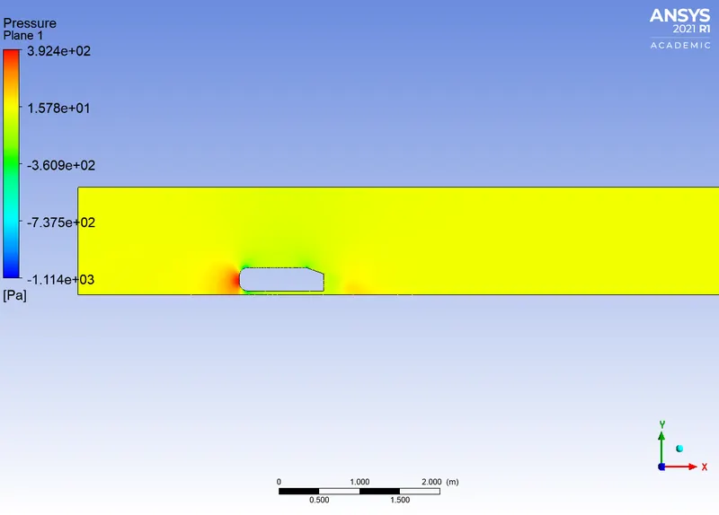
Pressure contour plane

Scaled Residuals plot

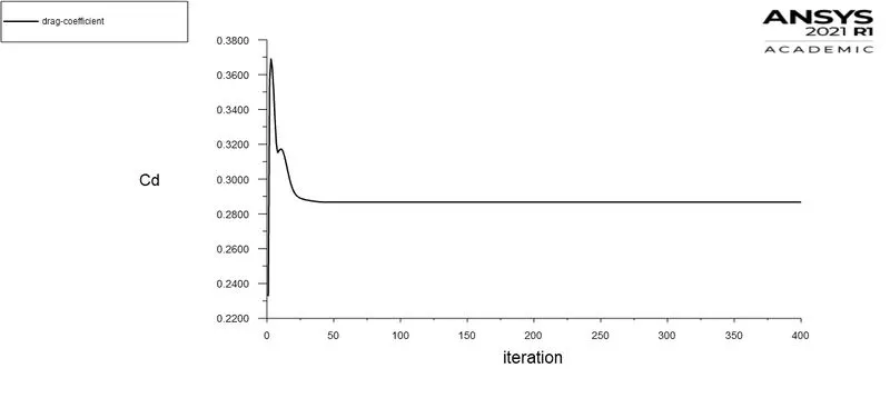
Drag coefficient plot

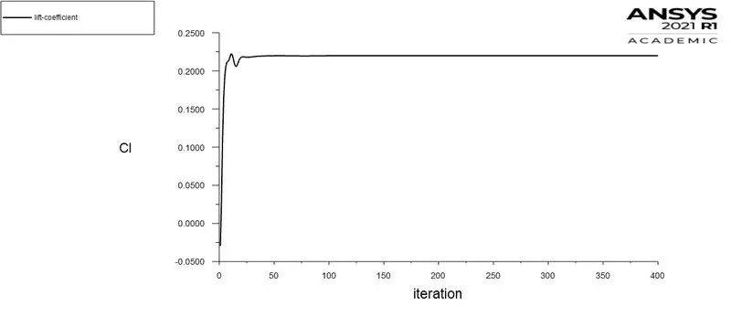
Lift coefficient plot

Vector plot clearly showing the wake region

Case 4:-

In the fourth case, the simulation was done with the following cell count;

• Y-plus = 10
• Viscous model: K-`omega`
• outer enclosure: 100 mm size of Hexahedral mesh
• inner enclosure: 35 mm size of tetrahedral mesh
• car body: 10 mm size of tetrahedral mesh
• inflation first layer thickness: 0.1428 mm
• No. of Elements: 439281
• Nodes: 118117

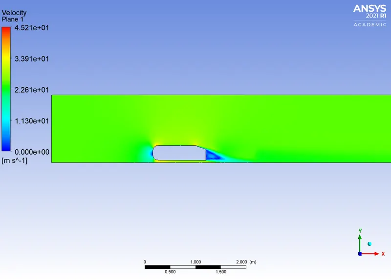
Velocity Contour plane

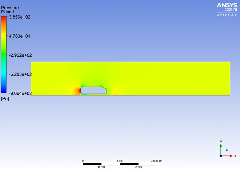
Pressure contour plane

Scaled Residuals plot

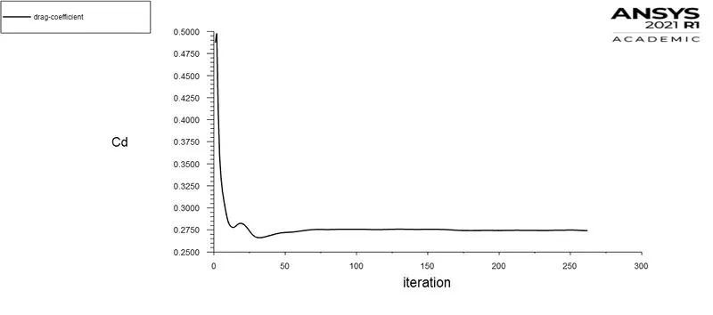
Drag coefficient plot

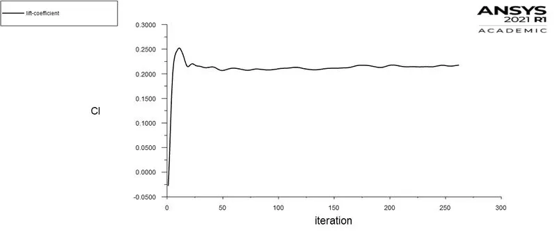
Lift coefficient plot

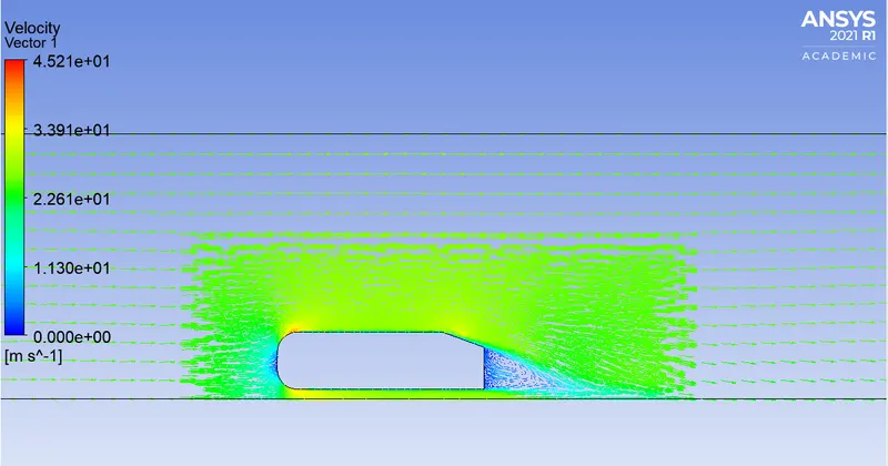
Vector plot clearly showing the wake region

Grid dependency test:

K-epsilon	No.of Elements	Nodes	`C_d`	`C_L`	Y+
CASE 1	329976	99226	0.2832	0.2397	50
CASE 2	384578	108773	0.3495	0.2782	100
CASE 3	372594	106763	0.2867	0.2198	125
K-Omega
CASE 4	439281	118117	0.2742	0.2174	10

CONCLUSION:

• Thus, we have created velocity contours and pressure contours for various mesh sizing and y+ plus values and also the vector plot clearly showing the wake region.
• The drag coefficient value for a refined case is 0.3495 which is around 0.33(Experimental value).
• It is clear that we have to maintain approximate `y^+` value to get correct value for drag coefficient.
• For `y^+` of 30-300, we have to use K-epsilon model to accurately predict the turbulent flow near the wall region of boundary layer.
• For `y^+` of less than 10, we can use K-omega viscous model (low Reynold's number model) to predict the turbulent flow region of near wall flows (should be meshed denser near wall). The k-ω model is similar to the k-ε model, but it solves for ω (omega) — the specific rate of dissipation of kinetic energy. It is a low Reynolds number model, but it can also be used in conjunction with wall functions. It is more nonlinear, and thereby more difficult to converge than the k-ε model, and it is quite sensitive to the initial guess of the solution. The k-ω model is useful in many cases where the k-ε model is not accurate, such as internal flows, flows that exhibit strong curvature, separated flows, and jets. A good example of internal flow is flow through a pipe bend.
• The omega can be integrated through the viscous sublayer without the need for a two-layer approach.
• There is a variation of pressure across the Ahmed body. The pressure in front of the body is positive because that's the location where the flow first comes in contact with the body and comes to rest. At the corner, the flow accelerates, thereby decreasing the pressure.
• The reason behind negative pressure in the wake region is due to flow separation, recirculating flow. It's a phenomenon that generally happens as the air moving past the body isn't able to pass through the immediate backside of the body creating a region, where there is no movement of air and thereby creating a pressure gradient.
• As the wake flow is the main contributor to the drag force(pressure drag), the point of separation is an important aspect of the flow. The more attached the flow is to the body the recirculation zone will be smaller and hence reduce the adverse effect of pressure drag, improving the fuel efficiency of the body.

REFERENCE:

1. Experiments and numerical simulations in the wake of a simplified car model.

https://www.researchgate.net/publication/330383775_Experiments_and_numerical_simulations_on_the_aerodynamics_of_the_Ahmed_body

2. Flow and Turbulence structures in the wake of a simplified car model.

https://www.researchgate.net/publication/266883948_Flow_and_Turbulence_Structures_in_the_Wake_of_a_Simplified_Car_Model_Ahmed_Model