Drop-test Simulation Report

Objective:

To simulate the fall of a cellphone on the floor using appropriate keywords in LS Dyna.

Case Setup:

ORIENTATION

The phone is oriented with respect to the floor such that the overhead section of the phone strikes the floor, as shown in the figure below

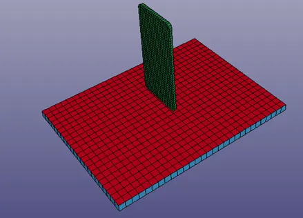
Figure 1 Isometric view depicting the orientation of the phone (green) with respect to the floor (red)

PARTS

Three parts are considered for the simulation:

• Phone (Solid part, Green)
• Floor Shell (Red)
• Floor Solid (Blue)

UNITS

The units considered for the simulation are SI units i.e. kg/m/sec.

MATERIAL

Two material models are considered for simulation

• Plastic Kinematic Material Model
• Rigid Material Model

Steel is considered as Plastic Kinematic Material with properties and parameters as provided:

• Density (RO) = 8050kg/m³
• Young’s Modulus (E) =210 GPa
• Yield Stress (S_y) = 700 MPa
• Tangent Modulus (ETAN) = 2.1 GPa
• Poisson Ratio (PR) = 0.3

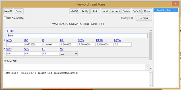
Figure 2 Steel as Plastic Kinematic material

The floor is modeled as a rigid material with the following properties:

• Density (RO) = 5000 kg/m³
• Young’s Modulus (E) = 1000 Gpa
• Poisson Ratio (PR) = 0.2
• CON1 = 7 (Constraint is applied in x, y, and z translation)
• CON2 =7 (Constraint is applied in x, y, and z rotation)

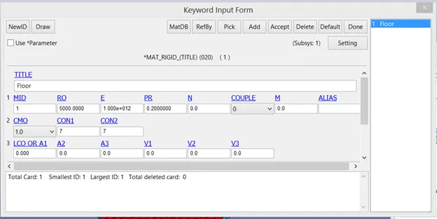
Figure 3 Floor as Rigid Material

SECTION

Phone and solid floor are modeled with solid section properties with ELFORM =1 (constant stress solid element), as shown in the figure below:

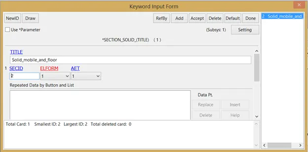
Figure 4 Section card for solid parts

Floor shell is modeled with shell section keyword with properties stated as follows:

ELFORM = 2 (Belytschko-Tsay (default))

Shell thickness (T1=T2=T3=T4) = 10 mm

NIP (Number of Integration Points) = 2

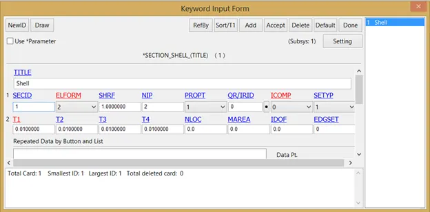
Figure 5 Shell Section card

INITIAL

Initial velocity is provided to the phone with this card under INITIAL_VELOCITY Keyword with initial velocity in negative z-direction = 5m/sec, shown in the figure below:

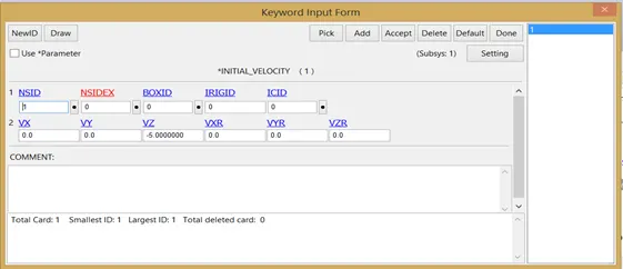
Figure 6 Initial Velocity applied to the phone via INITIAL_VELOCITY card

CONTACT

Contact between Phone (Solid) and Floor (Shell) is defined using Automatic Surface to the Surface contact card in Contact keyword, the parameters for the same are stated in the figure below:

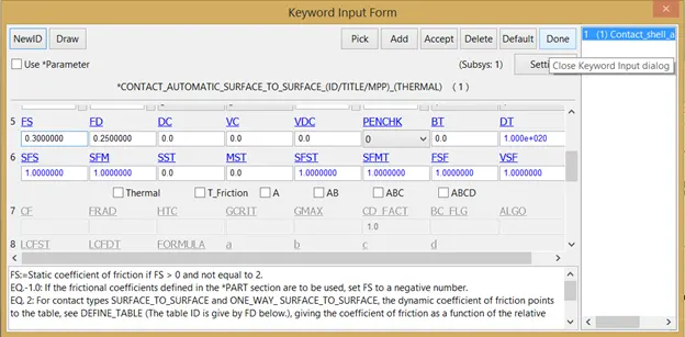
Figure 7 Automatic Surface to Surface contact card

Floor (Rigid Body) is treated as master surface, and Phone (Softer body) is treated as slave surface with static and kinematic friction values 0.3 and 0.25 respectively.

CONTROL

The termination time for simulation is defined using CONTROL_TERMINATION and is set to 10 seconds.

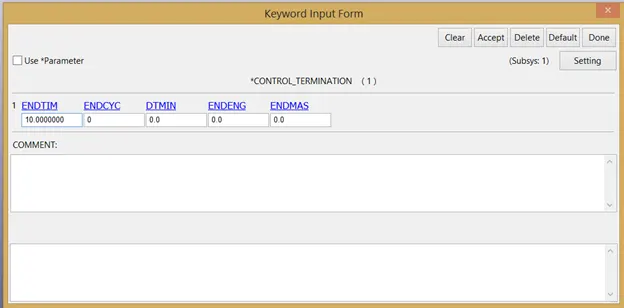
Figure 8 Determining simulation termination time using CONTROL_TERMINATION

The CONTROL_ENERGY (optional) card is used to compute various energies in GLSTAT and MATSUM, energies to be computed in the simulation are:

• HOURGLASS ENERGY (HGEN)
• STONEWALL ENERGY (RWEN)
• SLIDING INTERFACE ENERGY (SLNTEN)
• RAYLEIGH ENERGY (RYLEN)

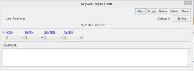
Figure 9 Includes various energies in calculation using CONTROL_ENERGY

HOURGLASS

An hourglass card is used to control the hourglass effect in simulation. Various parametric values defined for controlling the hourglass effect are set by default and are shown in the figure below.

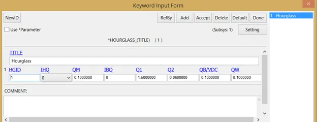
Figure 10 Hourglass card for controlling the hourglass effect

DATABASE

This card is utilized to plot the results of the simulation.

Various cards used are:

• BINARY_D3PLOT
• ASCII_GLSTAT
• ASCII_MATSUM
• ASCII_NODOUT
• ASCII_RCFORC
• ASCII_NODFOR

The data time interval between outputs is 0.1 sec for every output file.

Results

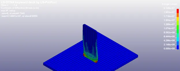
Figure 11 Illustration showing an instant of the impact of the phone with floor and von-mises stresses induced

GLSTAT

Using GLSTAT the energy plot of the system with time is plotted and shown in the figure below, various energies included in the plot are:

• Kinetic Energy
• Internal Energy
• Total Energy
• Hourglass Energy
• Damping Energy

As seen from the plot, the Kinetic energy of the system instantaneously drops to around zero at around 4 seconds, due to impact, and the hourglass energy increases dramatically due to stresses observed during impact.

The total energy remains conserved and the damping energy remains zero due to zero losses, and there is a spike in internal energy of the system during a collision.

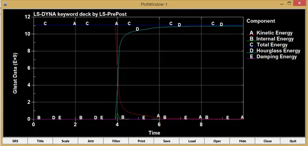
Figure 12 System energy plots using GLSTAT

Conclusion

The aim drop test was to test the LS Dyna environment for simulation regardless of the parametric values involved and the objective has been successfully achieved.

The results from the D3PLOT files have shown stress concentration on the corners of the edges of pone involved in the collision and thus the actual scenario has been successfully approximated in the simulation.

The k file of the drop test simulated has been attached with the submission.