Implicit vs Explicit FEM Solver

Both explicit and implicit solvers are two different methodologies to approach a solution for a given fem problem.

Explicit Solver

• The explicit solver relies on the explicit form of the FEM solution, such that the parameter to be evaluated in future time-step is separately defined as a function of the value of the parameter at present time-step.

For example:

G(t+dt) = F(G(t)),

Where g (t+dt) is the parameter to be evaluated at the successive time-step

And, g (t) is the parameter value at the present time step

• The solution obtained by the explicit solver is not inherently convergent in nature, as the explicit solver does not establish equilibrium between the internal and external forces at each time-step.
• The above limitation of the explicit solver is quantified in the form of Courant Friedrichs Levy criterion, according to which:

dt < L(ρ(1-2v)/2µ(1-v))^1/2

ρ is density of material

µ is shear modulus of material

v is wave velocity

dt is time-step size

L is edge length of element (references element size)

• This maximum time-step defines the time in which an elastic wave (impact wave) can travel through a single finite element of the model. Hence upper limit to the step size of time is defined, so as to obtain convergence through fem solution, and this method is conditionally stable.
• Application of explicit solvers is generally preferable to situations with highly transient behaviors (Dynamic Analysis) such as depicting significant jerk and acceleration and high strain rates example: explosive testing, impact testing, however, they can also be successfully employed to quasi-static conditions, but are not preferable for static conditions.
• LS Dyna is specially designed to solve Nonlinear Dynamic Transient analysis using explicit solver algorithms.

Implicit Solver

• The implicit solver relies on the implicit form of the FEM solution, such that the parameter to be evaluated in future time-step is not separately defined as a function of the value of the parameter at present time-step.

For example:

G(t+dt) = F(G(t)) + S(G(t+dt))

• In this form, the solution in successive time-step is a function of present and future timesteps, and thus due to matrix inversions involved in the solution, the calculation task becomes exhaustive.
• However, due to crosschecking of equilibrium at each timestep, this strategy is unconditionally stable and converges independently to the size of the timestep, hence a larger timestep can be considered.
• Application: The implicit solver is generally limited to static and quasi-static boundary conditions due to the large computational costs associated with it.

Explicit Solver	Implicit Solver
Faster Computation	Slower Computation
Conditionally stable due to timestep restraint	Unconditionally stable
Dynamic Analysis	Static and Quasi-Static analysis
Example: Impact Analysis, Explosive Analysis	Example: Static Structural Analysis

Aim

Use explicit and implicit methodologies to calculate the displacement in subsequent timesteps for the given force equation as f(u) = `u^3+9u^2+4u`, with incremental loading in both cases (tolerance provided for the implicit solver is 0.01 ). We will compare solutions obtained from both methodologies to the actual solution.

Explanation

The following terminologies are being utilized:

F is external applied load, t denotes time, and dt timestep size

f is internally evolved load

k is stiffness, R denotes the tolerance

u is displacement, du is displacement in the time interval

Assuming initial force and displacement to be zero and the incremental load in each timestep to be 4 units, this implies:

u₀ = 0, F₀ = 0 and dF = 4

f₀ = F₀ = 0, this implies R₀ = 0

Utilizing the equation df = k_i*du

Explicit Methodology

First iteration:

k₀ = (df/du)_u0, this implies k₀ = 4

du₁ = df/k₀, this implies du₁ =1

u₁ = u₀ + du₁, this implies u₁ = 1

k₁ = (df/du)_u1, this implies k₁ = 25

f₁ = ()_u1, his implies f₁ = 14

F₁ = F₀ + dF, this implies F₁ =4

R₁ = f₁ – F₁ = 10

Second iteration:

du₂ = df/k₁, this implies du₂ =0.16

u₂ = u₁ + du₂, this implies u₂ = 1.16

k₂ = (df/du)_u2, this implies k₂ = 28.9168

f₂ = ()_u2, his implies f₂ = 18.311296

F₂ = F₁ + dF, this implies F₂ =8

R₂ = f₂ – F₂ = 10.311296

Third iteration:

du₃ = df/k₂, this implies du₁ =0.13833

u₃ = u₂ + du₃, this implies u₃ = 1.29833

k₃ = (df/du)_u3, this implies k₃ = 32.427

f₃ = ()_u3, his implies f₃ = 22.552811

F₃ = F₂ + dF, this implies F₃ =12

R₃ = f₃ – F₃ = 10.552811

Fourth iteration:

du₄ = df/k₃, this implies du₄ =0.123353

u₄ = u₃ + du₄, this implies u₄ = 1.413353

k₄ = (df/du)_u4, this implies k₄ = 35.433

f₄ = ()_u4, his implies f₄ = 26.454

F₄ = F₃ + dF, this implies F₄ =16

R₄ = f₄ – F₄ = 10.454

For the above analysis I have utilized the below MATLAB script file to compute up to 10 successive time steps.

% explicit method for solvingg non linear dynamic problem, considering

% incremental loads

% given, u as displacement, f(u)is internal force

% k(u) as stiffness, F as external force

% f(u)= (u^3)+9(u^2)+4u;

% k(u)= f'(u)= 3(u^2)+18u+4;

% initial conditions are as follows

% initial displacement is zero u(1)=0;

% after each timestep, load increment is 4 unis, dF = 4;

u=zeros(1,10); dF=4;k=zeros(1,10);

F(1)=0;

for i=1:1:11

k(i)=(3*(u(i)^2)+18*u(i)+4);

du(i+1)=dF/k(i);

u(i+1)=u(i)+du(i+1);

f(i+1)=(u(i+1)^3)+9*(u(i+1)^2)+4*u(i+1);

F(i+1)=i*dF;

R(i+1)=f(i+1)-F(i+1);

end

Table 1 Iteration Table for explicit solver analysis

Timestep	du	u	F	f	k	R
0	0	0	0	0	4	0
1	1	1	4	14	25	10
2	0.16	1.16	8	18.3113	28.9168	10.3113
3	0.1383	1.2983	12	22.5527	32.4269	10.5527
4	0.1234	1.4217	16	26.7508	35.6538	10.7508
5	0.1122	1.5339	20	30.9192	38.6680	10.9192
6	0.1034	1.6373	24	35.0659	41.5141	11.0659
7	0.0964	1.7337	28	39.1959	44.2229	11.1959
8	0.0905	1.8241	32	43.3128	46.8164	11.3128
9	0.0854	1.9096	36	47.4191	49.3114	11.4191
10	0.0811	1.9907	40	51.5166	51.7206	11.6066

Implicit Methodology

The explicit solver calculations are performed in MATLAB through the script file code defined below:

%implicit method for solving non linear dynamic problem, considering

% incremental loads

% given, u as displacement, f(u)is internal force

% k(u) as stiffness, F as external force

% f(u)= (u^3)+9(u^2)+4u;

% k(u)= f'(u)= 3(u^2)+18u+4;

% initial conditions are as follows

% initial displacement is zero u(1)=0;

% after each timestep, load increment is 4 unis, dF = 4;

u=zeros(1,10); dF=4;k=zeros(1,10);du=zeros(1,10);f=zeros(1,10);R(1)=0;

F(1)=0;

for i=1:1:11

k(i)=(3*(u(i)^2)+18*u(i)+4);

du(i+1)=dF/k(i);

u(i+1)=u(i)+du(i+1);

f(i+1)=(u(i+1)^3)+9*(u(i+1)^2)+4*u(i+1);

F(i+1)=i*dF;

R(i+1)=f(i+1)-F(i+1);

k(i+1)=(3*(u(i+1)^2)+18*u(i+1)+4);

if abs(R(i+1))>0.01

while abs(R(i+1))>0.01

du(i+1)=-R(i+1)/k(i+1);

u(i+1)=u(i+1)+du(i+1);

f(i+1)=(u(i+1)^3)+9*(u(i+1)^2)+4*u(i+1);

R(i+1)=f(i+1)-F(i+1);

k(i+1)=(3*(u(i+1)^2)+18*u(i+1)+4);

end

else

end

end

Table 2 Implicit Solver Calculation table

Timestep	u	F	f	k	R
0	0	0	0	4	0
1	0.4722	4	4.0012	13.1691	0.0012
2	0.7244	8	8	18.6129	0
3	0.9169	12	12.0059	23.0274	0.0059
4	1.0772	16	16.0022	26.8709	0.0022
5	1.2170	20	20.0010	30.3499	0.0010
6	1.3422	24	24.0006	33.5643	0.0006
7	1.4563	28	28.0003	36.5753	0.0003
8	1.5616	32	32.0002	39.4253	0.0002
9	1.6597	36	36.0002	42.1372	0.0002
10	1.7517	40	40.0001	44.7374	0.0001

Plots

Figure 1 Displacement vs Force plot

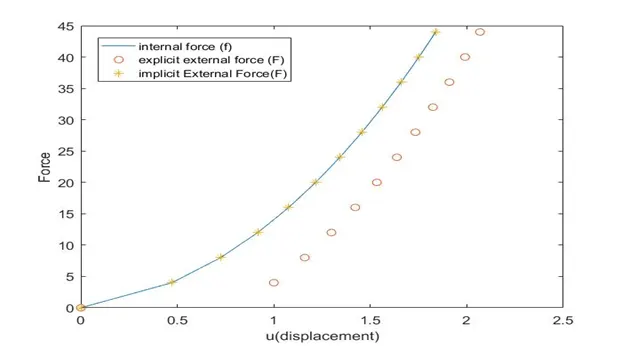
Figure 2 Time step vs Residual plot

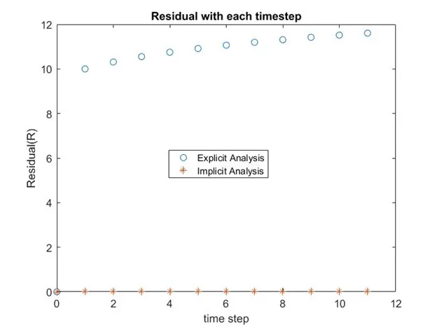
The above plot shows the force equilibrium in implicit analysis and the instability in the explicit analysis. As the residual tolerance limit in the implicit analysis is 0.01, the residual plot shows successful implementation of implicit solver code (with close to zero value for implicit analysis) so as to conform with an actual solution, however, the large residual values in explicit solution shows its departure from an actual solution.

Conclusion

The above plot shows the force equilibrium in implicit analysis and the instability in the explicit analysis. As the residual tolerance limit in the implicit analysis is 0.01, the residual plot shows successful implementation of implicit solver code (with close to zero value for implicit analysis) so as to conform with an actual solution, however, the large residual values in explicit solution shows its departure from an actual solution. Concluding, the implicit solution with provided tolerance works better with assumed timestep, however, there is an added computation cost, therefore with smaller load increments and timesteps better solution with explicit methodology can be obtained

Application

Application of explicit solvers is generally preferable to situations with highly transient behaviors (Dynamic Analysis) such as depicting significant jerk and acceleration and high strain rates example: explosive testing, impact testing, however, they can also be successfully employed to quasi-static conditions, but are not preferable for static conditions.

LS Dyna is specially designed to solve Nonlinear Dynamic Transient analysis using explicit solver algorithms.

The implicit solver is generally limited to static and quasi-static boundary conditions due to the large computational costs associated with it.

Explicit Solver	Implicit Solver
Dynamic Analysis	Static and Quasi-Static analysis
Example: Impact Analysis, Explosive Analysis	Example: Static Structural Analysis