Uniaxial Tension analysis of a test specimen

Aim

This report aims at analyzing the behavior of a cubical test specimen under uniaxial tensile load. The cards defined in the analysis are stated in the following section with a discussion on results in the final section of the report.

Case Setup

The preprocessing task for the analysis is defined in this section and the Ls Dyna cards utilized are defined accordingly:

1. Units

The units utilized for the task are:

Kg-mm-ms

2. 3D Modeling

As the test specimen geometry was a regular cube, the 3D model of the specimen was prepared in Ls Dyna.

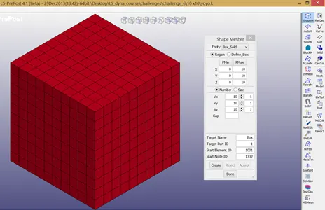
A 10x10x10 mm³ of geometry is created with 1000 solid elements of size 1x1x1 mm³ each.

3. Material Parameters

The material definition used for the test specimen is of hyperelastic material. The material card utilized is MAT_77 (O-Ogden_Rubber). As the material card definition was separately provided, the card was utilized in the main model file using the Include card.

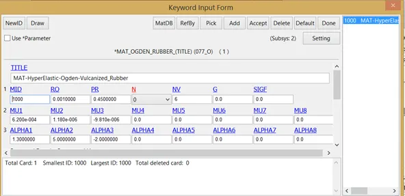
Figure 2 Material card parameters of MAT_77 (O-Ogden_Rubber)

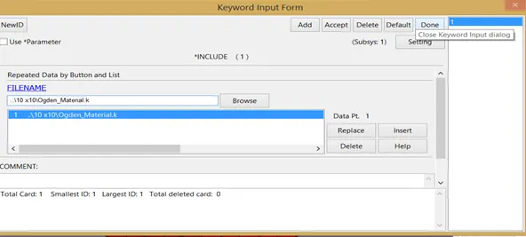
Figure 3 Include card to include the MAT_77 material card into the main model file

4. Boundary Conditions

Three boundary constraints were deployed along with one prescribed motion card to simulate the uniaxial tension conditions.

· SPC 1

The SPC 1 constraint was applied on all the nodes on the lower XZ face of the model.

The constraint was applied in

• Y-axis
• ROX
• ROY &
• ROZ

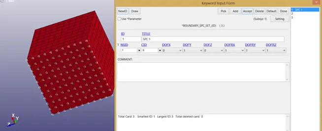
Figure 4 Highlighted nodes are the nodes subjected to SPC 1 constraint

· SPC 2

The SPC 2 constraint was applied on the nodes on the lower ZX face of the model along the central line parallel to the z-axis.

The constraint was applied in:

• X-axis

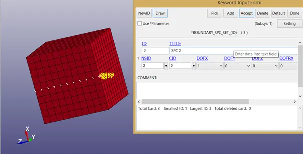
Figure 5 Highlighted nodes are the nodes subjected to SPC 2 constraint

· SPC 3

The SPC 3 constraint was applied on the nodes on the lower XZ face of a model, along the central line parallel to the x-axis.

The constraint was applied in:

• Z-axis

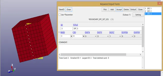
Figure 6 Highlighted nodes are the nodes subjected to SPC 3 constraint

· Prescribed Motion

All the nodes on the upper XZ face of the model are subjected to displacement along the +Y axis.

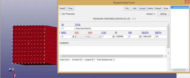
Figure 7 Highlighted nodes are the nodes subjected to boundary prescribed motion.

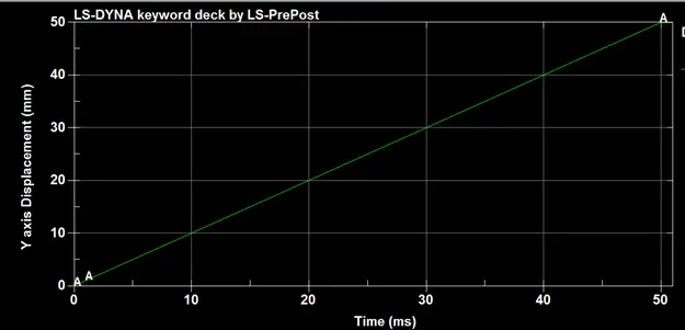
Figure 8 Y-axis displacement curve for boundary prescribed motion.

5. Control

This card is utilized to control the processing parameters of the problem.

The card used to control the analysis are:

· Control_Termination

This card is used to specify the problem run time. The run time of the problem is 51 ms.

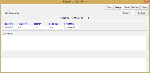
Figure 9 Control_Termination card to specify the termination time of the problem.

· Control_Timestep

This card is used to scale down the tssfac to 0.6 (so as to reduce the chances of instability and simulation errors).

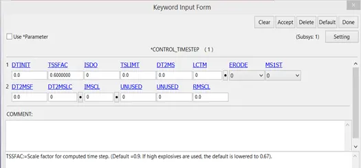
Figure 10 Control_Timestep card to specify TSSFAC.

· Control_Implicit_General

This card is used for switching to the implicit solver. For the cases where the implicit solver is used (IMFLAG = 1), else IMFLAG = 0.

6. Section

As described in the problem statement, the following elforms are used for defining section properties to solid elements:

• ELFORM = 1 (Constant Stress Solid Element)
• ELFORM = 2 (Fully Integrated S/R solid)
• ELFORM = -1 (Fully Integrated S/R solid intended for elements with poor aspect ratio, efficient formulation)
• ELFORM = -2 (Fully Integrated S/R solid intended for elements with poor aspect ratio, efficient formulation)

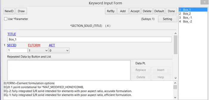
Figure 11 Section card for allocation of different section properties to solid elements.

7. Database

This card is utilized for post-processing purposes and result visualization.

Various sub cards utilized in database cards are:

· Binary_D3plot

This card is used for accessing visual information of the simulation results, i.e. visual comprehension of the model deformation during uniaxial loading. Also, it is used to include elemental and nodal, stress, and displacement behavior during analysis.

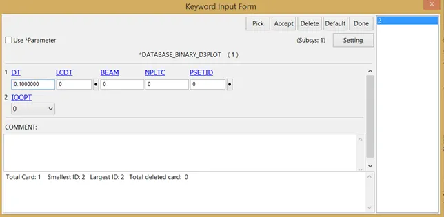
Figure 12 D3 plot card with DT =0.1

For the analysis, DT = 0.1, i.e. after each 0.1 ms of simulation time, a d3plot file will be written (having elemental and nodal properties of the specific timestep).

· Extent_Binary

This card is used to include the strain data in the d3plot file.

The STRFLAG is switched to 1, for including strain data into the d3plot file.

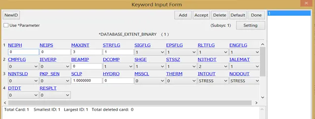
Figure 13 Extent Binary card with STRFLAG = 1, for adding strain data to d3plot

Results

The analysis was carried out with explicit as well as an implicit solver for all the ELFORM options described in the problem statement (ELFORM = 1, 2, -1, -2). For evaluating stress vs stretch ratio plots central element of the 3D model was selected (Element no. 456). The selection of Element no. 456 is because the element is centrally located in the model. However, the credibility of this selection will be discussed in the latter part of the result section.

1. Explicit solver results

The solver was run with Control_Timestep_TFFAC = 0.6 (to reduce chances of numerical instability).

Although the processing time with explicit solver was significantly less (around 10 seconds for each problem), however as shown in the figure, the plots show dissimilarity with the actual plot defined in the problem statement. Further discussion on explicit solver results is abandoned due to dissimilarity from actual results.

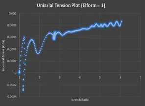
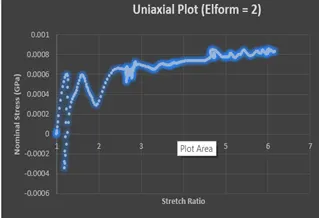
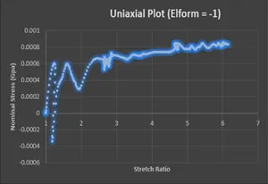
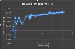
Figure 14 Uniaxial tension Plot for Element no. 456 with explicit Solver and Elforms 1, 2, -1 & -2 respectively

2. Implicit solver results

IMFLAG was switched to 1 in Control_Implicit_General, for problem processing with the implicit solver. The influence of the selection of ELFORM for the implicit case setup proved insignificant as the results were quite similar.

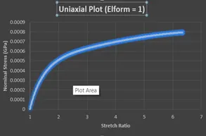
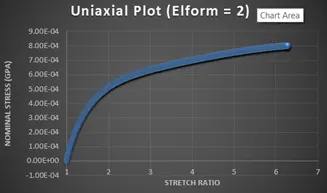
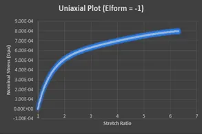
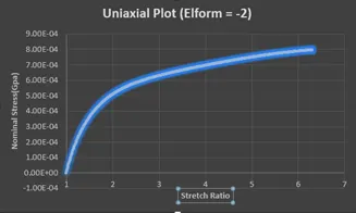
Figure 15 Uniaxial tension Plot for Element no. 456 with implicit Solver and Elforms 1, 2, -1 & -2 respectively

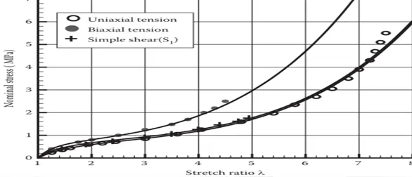
Figure 16 Actual material behavior plot provided in the problem statement

However comparing to the actual plot, the implicit solution plots show a similar trend. Comparison of the actual plot with the simulation result reveals the following points:

• The actual plot has more curvature after the initial bend while the implicit solution plot is straighter after the first bend.
• The inconsistency in the results increases as the stretch ratio extends beyond 5.

Inconsistency in results is probably due to the following reasons:

• Failure of material model parameters to simulate exact material behavior (Especially at higher stretch ratios)
• Mesh convergence not achieved.

3. Credibility of element selection

One of the central elements (Element no. 456) of the model was selected for the plot. The justification of the selection of the central element owes to the fact that in uniaxial tensile loading, stress vs strain plots are evaluated at the central portion of the specimen.

To check the variance in stress-strain plots among different central elements following graphs were plotted.

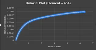
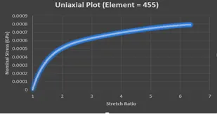
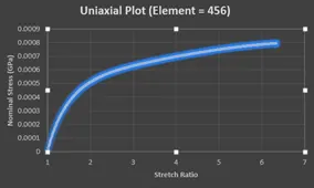
Figure 17 Nominal Stress vs Stretch Ratio plots of Elements 454, 455 & 456 respectively for Implicit analysis with ELFORM =1

The above plots reveal that all nearby elements experience the same stress (approx.) for a given stretch ratio. Hence the arbitrary pick of any central element is validated as all elements behave similarly.