Week - 3 Drop test Challenge

Challenge 3 - Cellphone Drop Test

Objective

Perform a complete simulation of a cellphone drop test, which will require to:

• Create a material card with aluminum properties
• Create a rigid wall to mimic ground
• Assign proper boundary conditions
• Define contacts between the cellphone and ground
• Define proper outputs in form of both binary D3 plots and ASCII file

Procedure

The first step is to import the model to LS-PrePost, which can be done using the "import Ls-Dyna keyword file" option

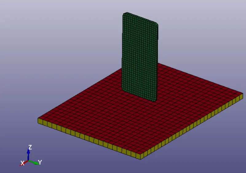
We can observe that we have a total of 3 parts in the model, the cellphone, ground and a layer of shell elements, which we will proceed to delete since we will apply a rigid wall definition as the ground

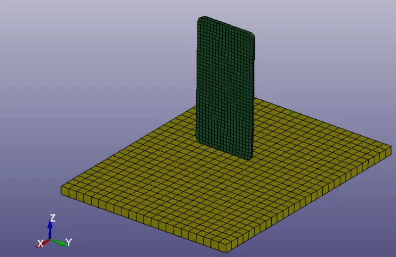
Once this is done we can start by defining material properties for both the cellphone and the ground.

The cellphone material will be considered as Aluminum 6061, whose material properties are shown below:

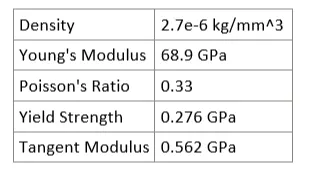
To keep consistency in the model we will use the Kg/mm/ms unit system

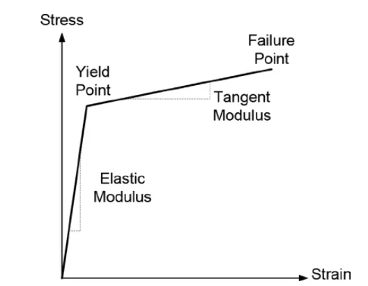
By specifying the tangent modulus and using the MAT_024 model, we can define an elastic-plastic material that provides a stress-strain distribution given by:

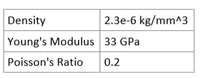
Meanwhile, the ground will be defined by using a MAT_020 rigid body material. We will use concrete material properties as given by the next table:

In order to assign these material models to their corresponding parts, we first must create Section cards which contain the element formulation (constant stress solid element)

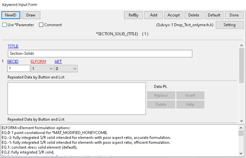
Then, we can proceed to assign both the section card and the material in the PART module.

The next is to apply the boundary conditions in the model. To do so, we must create two separate Node Sets to distinguish between the elements of the ground and the cellphone.

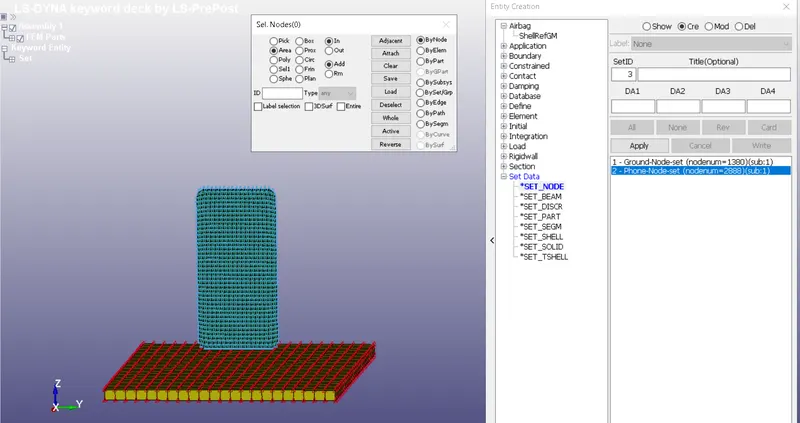
From there, we can use the option "Create Entity --> Boundary ---> SPC ---> All Fix" to mimic ground

For the cellphone, we will do a similar procedure but we will an initial velocity keyword. The initial velocity can be calculated using the following kinematic equation:

Assuming an initial velocity of 0 mm/s, and a height of 2,000 mm we get:

Due to the global coordinate system position, this velocity has to be applied in the -Z direction

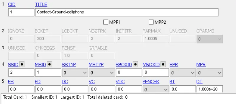
The next step is to define contact between the cellphone and ground so that we avoid a situation in which the phone nodes passes through the other body. To do so, we must create Set Data Segments which contain the nodes that will be interacting.

For the ground, we will select a square section that covers the area of the phone, and for the cellphone we will select all the nodes in the body

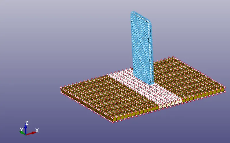
From there we can proceed to define the contact. This can be done using the AUTOMATIC_SURFACE_TO_SURFACE contact definition. We must remember to mark the ground as the Master, and the Phone as the slave

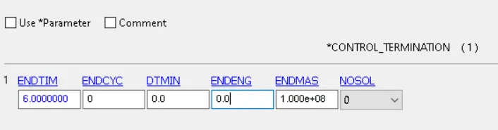
The next step is to assign the control termination card, in which we will define the duration of the simulation. Knowing that the distance from the phone to the ground is approximately 30mm, and dividing over our initial velocity we get:

To ensure proper results, we will input a 6 ms time for the simulation

The last step is to define the output database as both binary D3PLOT and ASCII files. This option will allow us to visualize the stress/strain distribution in the component, as well as the energy summary during the simulation

We will choose to plot the results (Using the binary D3PLOT) every 0.1 ms

In terms of the ASCII options, we will choose to record the following:

• GLSTAT ---> Energy summary of the simulation
• MATSUM --> Specific material energy
• RCFORC ---> Resultant internal and contact forces
• NODOUT ---> Nodal point data
• RWFORC ---> Rigid wall forces

Once these are defined, we can run the simulation using LS-Run and open the binary file to post-process the results

The first thing we have to do is to check for the energy balance during the simulation. Using the GLSTAT output, we can plot for the kinetic, internal and hourglass energy, obtaining:

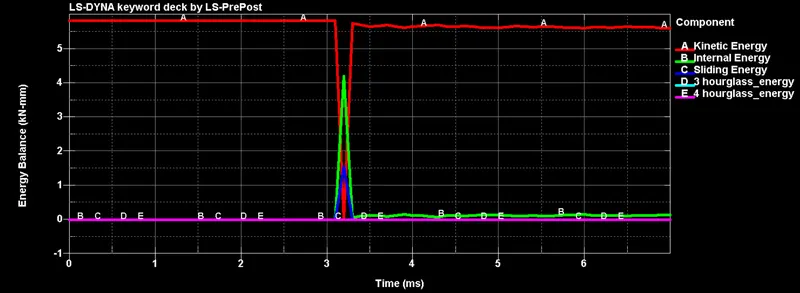
The expected kinetic energy in the model can be calculated analytically as:

As observed in the graph, this energy gets converted into internal and sliding energy at the moment of impact, and then fully converted to kinetic when the cellphone bounces back. It's also worth noting that the hourglass energy remains neglectable during the entire simulation

The next step is to check for both the stress and strain contour plots, which have the following distributions at the moment of impact:

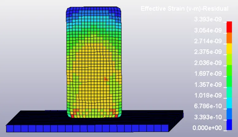
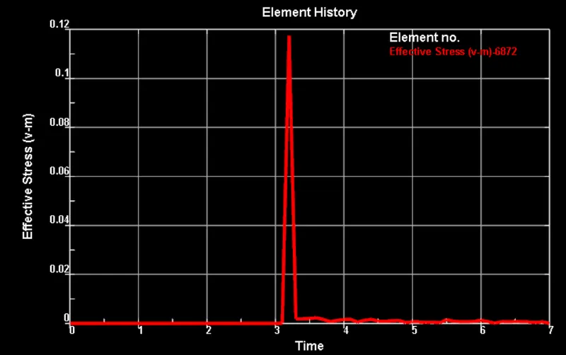
As expected, the stresses and strains in the phone follow the same distribution with time, with the most affected elements being before the corners of the model, and from there a uniform stress distribution up to the top. The maximum stress developed in the model corresponds to 0.12 GPa, which is below the yield strength of the material. This only occurred because the phone impacts the ground without any angle.

Link to stress contour Animation:

https://drive.google.com/file/d/17ILDDZRUUP3-_zuj378WZQIBq_Pasl2E/view?usp=sharing

Conclusions

• All the stresses/strains developed during the simulation are in the elastic range
• All the kinetic energy was successfully converted into internal and sliding energy
• Hourglass energy was kept at 0 due to proper element formulation