Drop test on Cell Phone Structure using LS-DYNA

INTRODUCTION

Drop test is among the significant test for the cell phone industries. The cell phone is tested by dropping it from various angles to check its survival against damage. It is done to investigate the weaker zones of the mobile, due to which the cell could damage. To save the time and the capital required to do the actual test, the industry prefers to do the virtual simulations at the design stage. In this work, an explicit analysis was performed on a cell phone for a few milliseconds. The analysis was explicitly performed to see the behavior and the damage on the cell, milliseconds before and after impact. The time from when the cell phone drops from hand to just before touching the floor is not considered.

OBJECTIVE

• To create a complete simulation file to perform a drop test on a cell phone.

PRE-PROCESSING

In the LS-PrePost application, using the File → Open → LS-DYNA Keyword File, the keyword file is input. A discretized model of cell phone was only available as a keyword file to input in LS-DYNA. The input model can be seen in fig. 1 below.

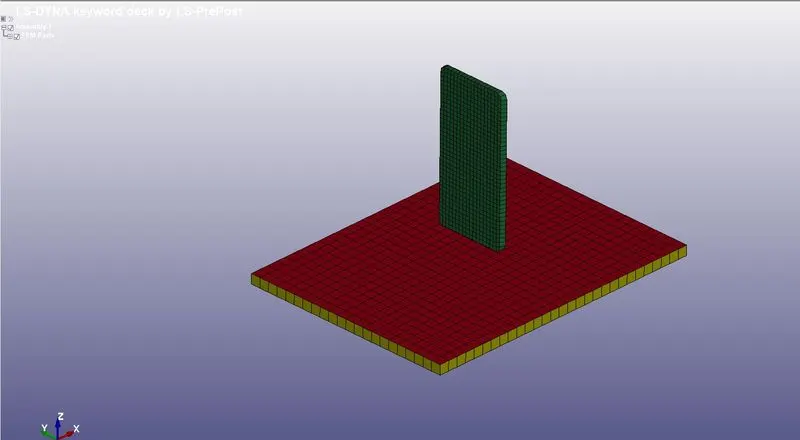
Figure 1: The discretized model of cell phone and floor.

In fig. 1, in the left-upper corner, the title name can be observed as ‘LS-DYNA keyword deck by LS-PrePost’. To change this title first, the keyword file was opened in Notepad. It appeared as shown in fig. 2.

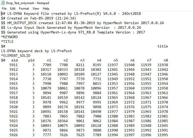
Figure 2(a): Keyword file opened in Notepad application.

In fig. 2(a), the TITLE can be observed written as ‘LS-DYNA keyword deck by LS-PrePost’. Thus, in Notepad itself, the title was changed to ‘Cell Phone Drop Test’. Also, the KEYWORD was changed to KEYWORD_ID and was given the name ‘CELL_PHONE_DROP_TEST’. Space between characters is not allowed in keywords. The updated file can be seen in fig.2(b) below.

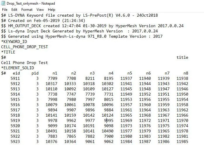
Figure 2(b): Updated keyword file in Notepad.

Now when this updated file is opened in the LS-PrePost application, the change can be observed in fig. 3. The title name now has changed to ‘Cell Phone Drop Test’. Also, when the simulation will run, all the output files will be generated with the name ‘CELL_PHONE_DROP_TEST.format’.

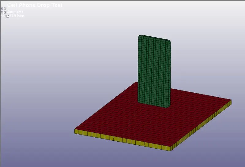
Figure 3: The title has changed to ‘Cell Phone Drop Test’.

Fig. 4 below shows the Keyword manager dialog box. It includes some keywords like ELEMENT, KEYWORD, NODE, PART, TITLE. These are the basic keywords that are always present when a model has discretized in one software and then opened in LS-DYNA.

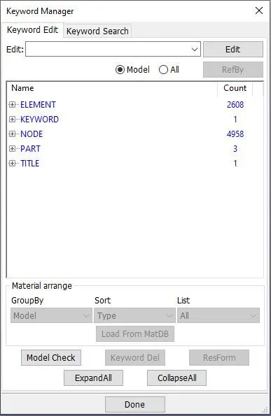
Figure 4: Keyword Manager dialog box.

• Material Definition

The cell phone industry generally follows the (gm, mm, ms) unit to simulate the model. Therefore, in this work, the same unit is followed. According to it, for steel material, the density is equal to 7.85e-3 gm/mm³, young’s modulus is equal to 210*10³ (gm/mm.ms²), the yield stress is equal to 250 (gm/mm.ms²), and Poisson's ratio is equal to 0.3.

For a concrete material, density is equal to 2.5e-3 gm/mm³, young’s modulus is equal to 210*10³ (gm/mm.ms²), and Poisson's ratio is equal to 0.2

Now to create all the conditions for simulating the model, it starts with defining a material. Thus, in keyword manager, picking ‘All’ and selecting ‘MAT → 024-PIECE_LINEAR_PLASTICITY’ a plastic material card was selected. The plastic material card is used to check the damaged regions of the model whose stress is above the yield point of the material, and ignore the stresses that are below the elastic limit. It is based on the yield stress and plastic strain to failure of the material. The material card for the deformable model is as shown below.

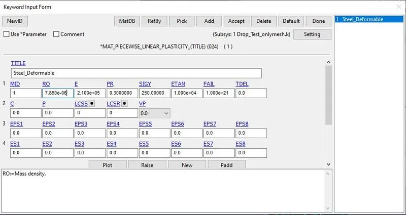
Figure 5: Material card created for deformable-body i.e. the cell phone.

The values of the material card were based on the data provided. Once the material card is created, in the part card of cell phone, the material id of this material is provided to it.

Similarly, another material card was created by selecting the card ‘020-Rigid’. The mechanical properties of concrete were provided to this card, with a material 2 (earlier material id was 1). Also, its deformation was constrained from all directions. Once created, this material was assigned to the floor part of the model.

• Section Definition

After material definition, the next necessary thing is to define the section. Defining the section means defining the elemental property, that how should the elements behave, and how many integration points they would have.

In this model, both the cell phone and the floor consisted of only solid elements. Therefore, only one section id was created for both parts. In the Keyword Manager, again picking the ‘All’, and in SECTION, the SOLID was selected.

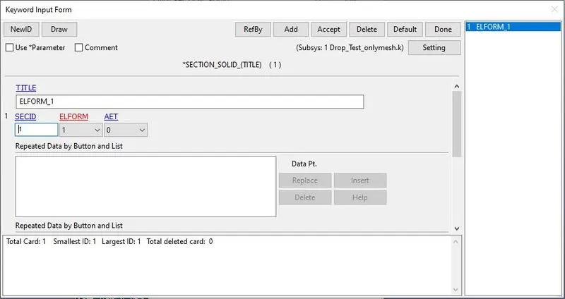
Figure 6: Solid Section Card to define the ELFORM = 1 for all the solid elements.

As can be seen in fig. 6, in the SOLID card the SECID or section id was given as 1, and the ELFORM or the element formulation was selected 1. It ensures constant stress in solid elements.

Once created, this SECTION was assigned to both the parts using its section id.

• Contact Definition

When the simulation would occur, the cell phone would come in contact with the floor. Thus, a contact definition was required. This ensured that the impacting part will not pass through, and will be pushed back out of the master segment.

To define the contact, the first set of parts was required to create. Therefore, using Create Entity → Set Data → *SET_PART, two sets were created each for the cell phone and the floor.

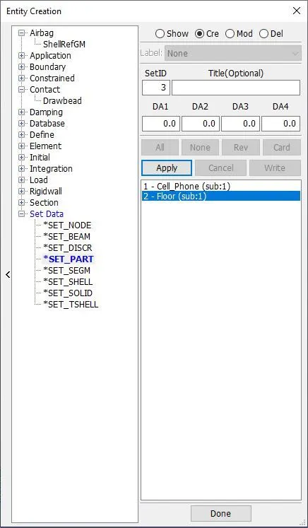
Figure 7: Two separate sets created for cell phone and the floor each.

Now, to define surface-to-surface, in the keyword manager picking the ‘All’, in the CONTACT, AUTOMATIC_SURFACE_TO_SURFACE was selected. In that, at first SSTYP and MSTYP were selected as 2, which allows selecting the set by part. The in SSID, a set of cell phone part was selected to make it a slave body, and in MSID, a set of floor part was selected to make it a master body.

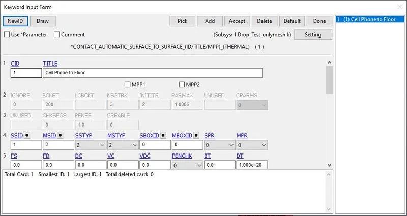
Figure 8: Contact Card was created to define surface-to-surface contact between cell phone and the floor.

• Boundary Condition

Once the model is ready with the material, elemental formulation, and contact, it is ready to define the boundary condition. In boundary conditions, the cell phone had to provide an initial velocity of 10 mm/ms in a vertically constrained direction (as per the data provided). Thus, to do this, firstly, a set of nodes was required. Therefore, using create entity → Set Data → *SET_NODE, a set of nodes was created for cell phone.

Now, to give the initial velocity of 10 mm/ms to the cell phone, in the Keyword Manager, picking the ‘All’, INITIAL → VELOCITY was selected. In that velocity card, the nodal set id was selected that was created just earlier, and VZ is given as -10 to provide the initial velocity of 10 mm/ms in a vertically downward direction.

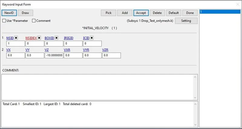
Figure 9: Initial Velocity card to give the initial velocity of 10 mm/ms to the cell phone in a vertically downward direction.

• Control Cards

The control cards are required to control the simulation process. In this, the most essential card that is required is the termination card. It is used to define the termination time of the simulation. The distance between the floor and the closest node of the cell phone was around 20 mm. The velocity provided was 10 mm/ms. Thus the total time required for the cell phone to touch the floor is around 2 ms. Therefore, the termination time can be set around 3.0 ms. It was defined using the Keyword Manager, picking the ‘All’ and selecting CONTROL → TERMINATION. In that card, the ENDTIM or the end time was given as 3.0.

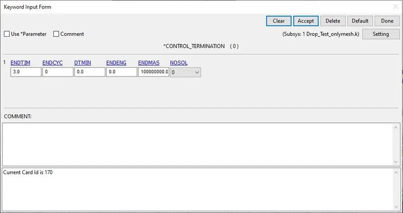
Figure 10: Card to define the termination time.

• Database Cards

Database cards are required to command the software that what files are required as output. In this simulation, binary_d3plot was required to generate. So using Keyword Manager, and selecting the ‘All’, in the DATABASE, BINARY_D3PLOT was selected. In that card, DT was given as 5e-4, which plots the results at every 5e-4 milliseconds.

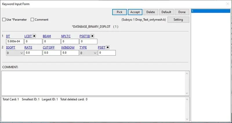
Figure 11: BINARY_D3PLOT card.

In the results, since the energy behavior is the part of the concern, in ASCII, a GLSTAT card was required to activate. ELOUT was also activated to get the element output data. To activate them, in the Keyword Manager, picking the ‘All’, in DATABASE, ASCII_option was selected. In that card, GLSTAT and ELOUT were activated, providing the DT value of 5e-4, to print the results at every 5e-4 milliseconds.

Next, to get the history of behavior of any element of the cell phone, the HISTORY_SOLID card was required. Thus, using the same procedure as followed before, in the DATABASE, HISTORY_SOLID was selected. In that card, two elements were selected, of which history was required.

Once done with defining the keywords, the next essential thing is to check that if any errors are present in it. Therefore, using the Model Checking, the keywords were checked for errors and warnings. As can be seen in fig. 12, no error and warning was found in the defined keywords.

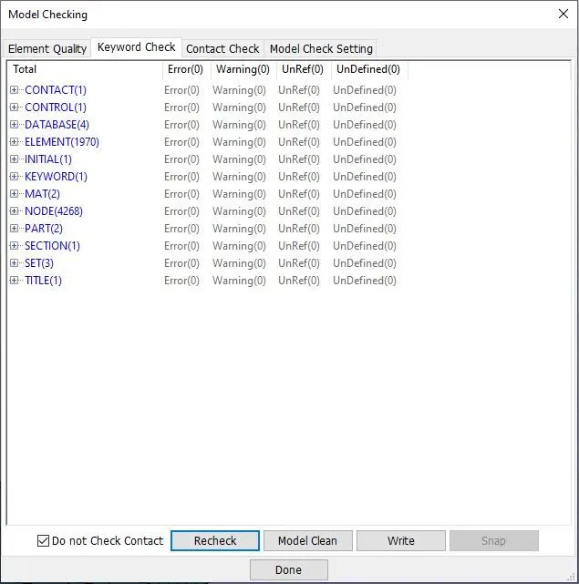
Figure 12: Model Checking to check the errors in the keywords.

After completing defining all the keywords, the model was saved in .k format.

SOLVING

When the model is all set with material, element formulation, contacts, boundary conditions, and simulation control setup, the model is ready for the simulation. To run the model, the model was first saved in .k format. Using the LS-Run application, the .k file was imported to it and ran the simulation. The run terminated normally, and the output file has shown that the run took 14 seconds for solving.

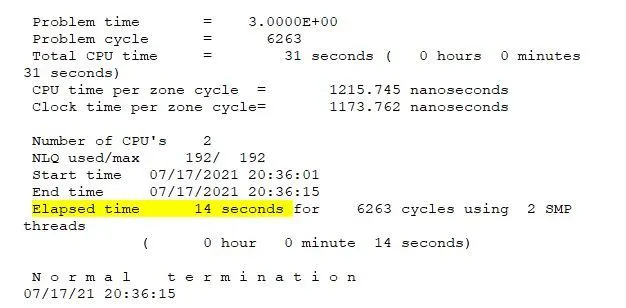
Figure 13: Output file showing the elapsed time of 14 seconds, with normal termination.

POST-PROCESSING

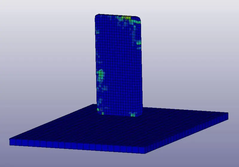
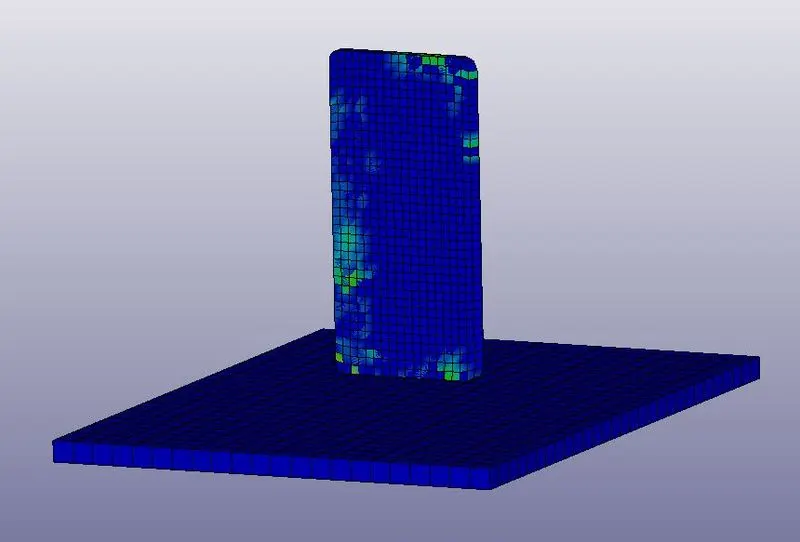
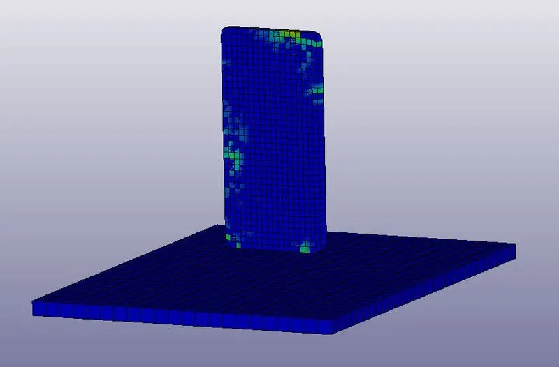
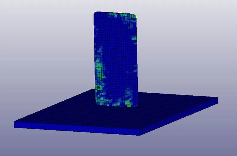
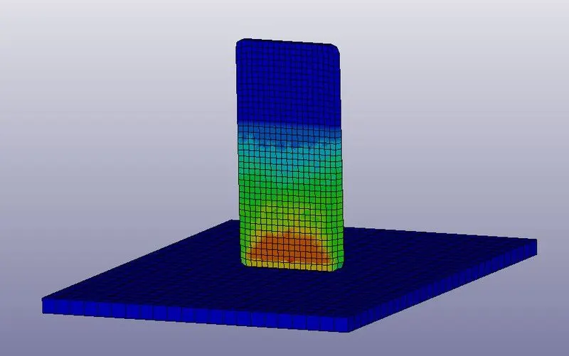
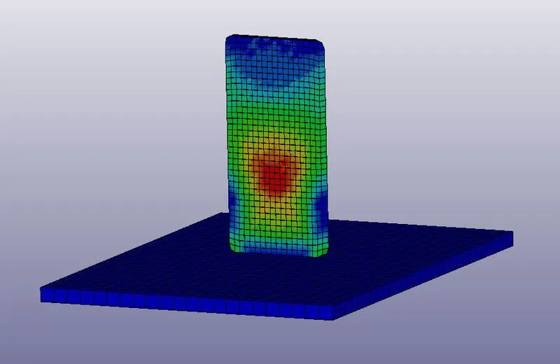
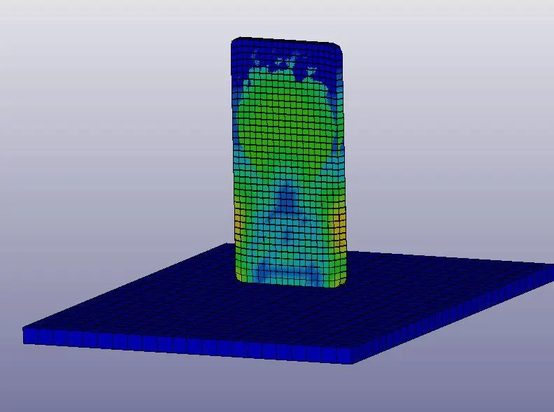
After solving, the .d3plot file was imported in the LS-PrePost application. The von-mises result at various time intervals can be seen in the figure below.

at 0.505 ms	at 0.999 ms	at 1.000 ms
at 1.516 ms	at 2.000 ms	at 2.516 ms
at 3.000 ms

Figure 14: Von-mises stress behavior at various time intervals.

In the von-mises result itself, it can be observed that when the cell phone is impacted with at 2.000 ms a sudden increase in stress occured at the floor and cell phone contact. The maximum stress at 2.000 ms was 254.3 MPa, which is just above the yield strength. But at 2.044 ms the maximum stress level was increased to 314.1 MPa, which is a significant value to consider. If the value had remained at around or below yield strength the model could be considered safe in the drop test. But this significant increase in the stress shows that more design modification is required, which would reduce this stress level. Fig. 15 shows the von-mises or effective stress vs. time plot for the element on the lower side of the cell phone.

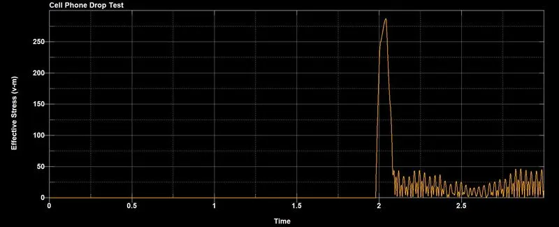
Figure 15: Effective stress vs. time plot for the element on the lower side of the cell phone.

Fig. 15 shows that the effective stress suddenly increased as the cell phone came in contact with the floor just before 2 ms, and it increased above 300 MPa, which is not acceptable.

Fig. 16 shows the kinetic energy and internal energy plot vs. time. The sudden drop in the kinetic energy when the cell phone impacted with floor increased the internal energy.

Ideally, after impact, the internal energy has to be equal to the kinetic energy, but the difference between the internal energy and the kinetic energy could have transferred as thermal energy or contact energy.

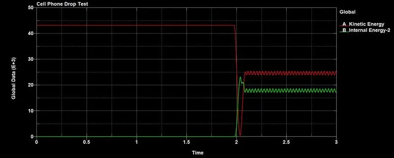
Figure 16: Kinetic Energy, and internal energy vs. time plot.

CONCLUSION

The cell phone model was analyzed for the drop test against floor. In the drop test, instead of gravity an initital velocity of 10 mm/ms was provided to it. The simulation was set to terminate at 3 ms. The run took 14 seconds to solve the problem. In the results, it was found that the maximum stress generation in the cell phone is above 300 MPa, which is not acceptable. The value has to be close or below yield strength value i.e. 250 MPa. Thus, the simulation suggests a requirement of significant modification in the cell phone.