Week-3 Challenge: ADVISOR Tool
TASK-1
SIMULATION USING ADVISOR TOOL
AIM: To Simulate the EV_defaults_ in file using ADVISOR tool for the given conditions.
OBJECTIVE: Simulate the EV_defaults_in vehicle model with the FTP Drive cycle and need to find the following things.
- Can the vehicle travel 45km by changing the cargo mass to 500kg and all other conditions are default.
- Repeat the simulation by changing the battery capacity and other conditions same as above case.
DESCRIPTION:
ADVISOR TOOL
Advanced Vehicle Simulator (ADVISOR) was first developed in November 1994 at the National Renewable Energy Laboratory. It was designed as an analysis tool to assist the US Department of Energy (DOE) in developing technologies for hybrid electric vehicles (HEV) through the Hybrid Electric Vehicle Propulsion System contracts with Ford, General Motors, and DaimlerChrysler. Its primary role is to highlight the system-level interactions of hybrid and electric vehicle components and their impacts on the vehicle performance and fuel economy.
ADVISOR was created in the MATLAB/Simulink environment. MATLAB provides an easy-to-use matrix-based programming environment for performing calculations while Simulink can be used to represent complex systems graphically using block diagrams. ADVISOR uses three primary graphical user interface (GUI) screens to guide the user through the simulation process. With the GUIs, the user can iteratively evaluate the impacts of vehicle parameters and drive cycle requirements on the vehicle performance, fuel economy, and emissions. The GUIs facilitate interaction with the raw input and output data that is present in the MATLAB workspace. The vehicle model is depicted graphically using Simulink block diagrams to define the connections between components. The model then reads the input data from the MATLAB workspace during the simulation and outputs the results to the workspace to be viewed in the results window.
1. EV_defaults_in
- Open the ADVISOR tool
- After opening the ADVISOR tool, we can observe that the default loaded file will be PARALLEL_defaults_in.
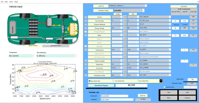
- From the option load file change the vehicle input to EV_defaults_ in and the file will be loaded.
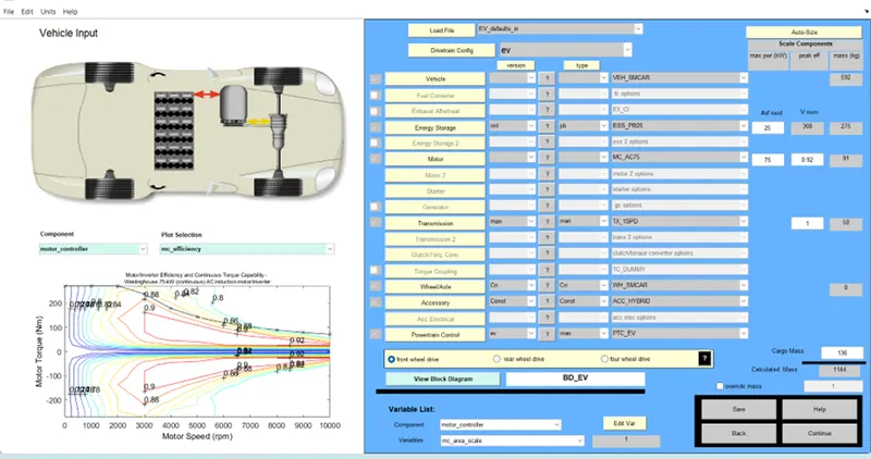
- We can observe the initial default conditions of EV_defaults_in
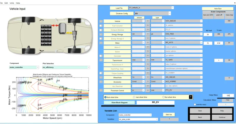
Mass of the Vehicle body = 592 kg
Cargo mass = 136 kg
No. of battery modules = 25
Nominal voltage of Battery pack = 308v
Mass of the battery pack = 275 kg
- Then we need to change the drive cycle to CYL_FTP, the default No. cycles was set to 1 and run the simulation.
CYL_FTP Drive Cycle
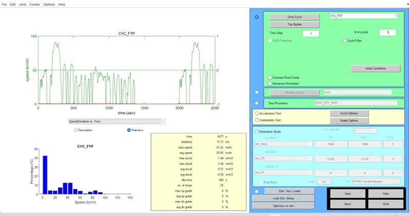
- We can observe that the distance travelled by the vehicle for One Was 17.8 km and the SOC state of battery reaches to 67.5%.
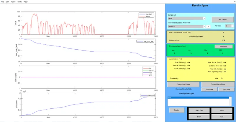
- We need to change the cargo mass of the vehicle to 500 kg and continue the simulation.
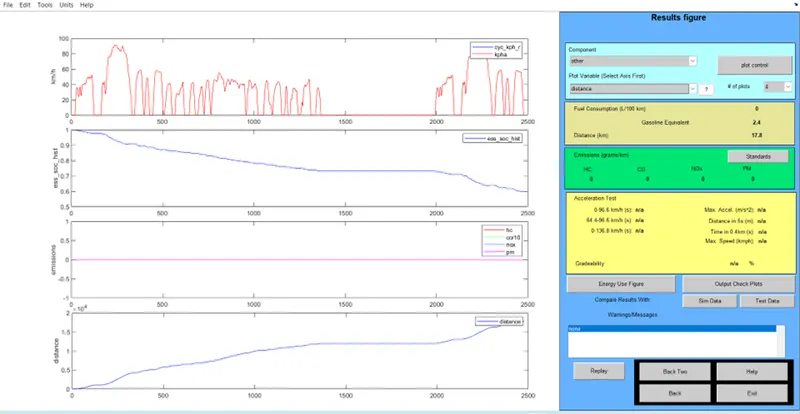
- Then distance travelled by the vehicle for One Was 17.8 km and the SOC state of battery reaches to 60%.
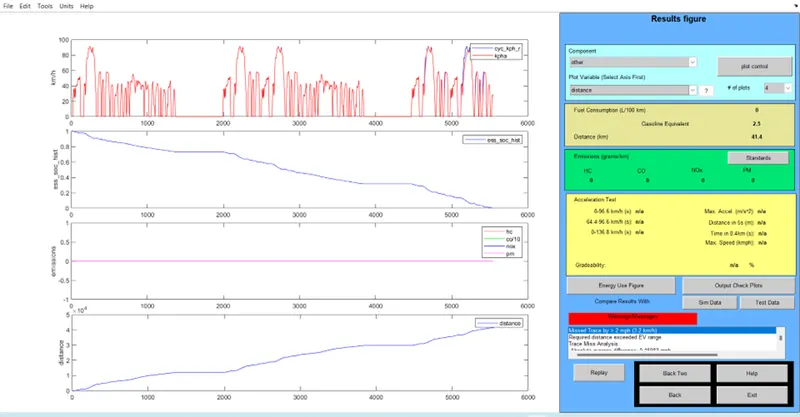
- Now we increased the No. of drive cycles to 3, to check the total distance travelled by the vehicle.
- After running the vehicle for 3 cycles of FTP we can observe that the SOC state of the battery reaches to zero even before completing the third cycle i.e., approximately at 5500s.
- The distance travelled by the vehicle is 41.4km.
2. Change in Battery Capacity.
- We need to change the battery capacity for the above case and run the simulation again.
- We can observe that from the above case
Mass of the Vehicle body = 592 kg
Cargo mass = 500 kg
No. of battery modules = 25
Nominal voltage of Battery pack = 308v
Mass of the battery pack = 275 kg
- We increased the No. of battery modules to 26 from 25.
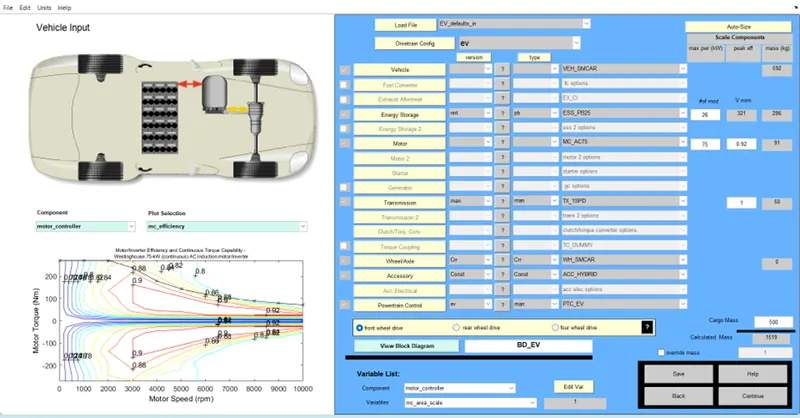
- We can observe that the nominal voltage of battery pack increased to 326v and the weight of the battery pack to 286 kg.
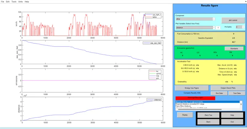
- After running the vehicle for 3 cycles of FTP we can observe that the SOC state of the battery reaches to zero even before completing the third cycle i.e., approximately at 5800s.
- The distance travelled by the vehicle is 42.7km.
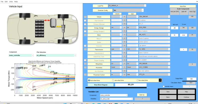
- We increased the No. of battery modules to 28.
- We can observe that the nominal voltage of battery pack increased to 345v and the weight of the battery pack to 308 kg.
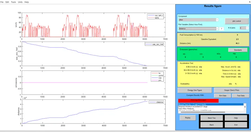
- After running the vehicle for 3 cycles of FTP we can observe that the SOC state of the battery reaches to zero even before completing the third cycle i.e., approximately at 6100s.
- The distance travelled by the vehicle is 46.3km.
OBSERVATION:
- From the above two experiments we can observe that if the mass of the vehicle increases the distance travelled by the same vehicle for the same battery capacity, will be decreased
- If we increase the nominal voltage of the battery pack by increasing the No. of modules in the battery the distance travelled by the vehicle may increase but the weight of the battery pack also increases with the increase in the battery pack
CONCLUSION:
- From the above experiments I can conclude that while we modelling an EV or HEV we need to check with the distance needs to be travelled by the vehicle, the cargo mass and the battery pack capacity.
- If we wants to travel more distance with high cargo mass we need more battery pack capacity if we increase battery pack then total weight of the vehicle body increases.
TASK-2
GRADEABILITY TEST USING ADVISOR TOOL
AIM: To Simulate the PRIUS_Jpn_defaults_in file using ADVISOR tool for the given conditions.
OBJECTIVE: Simulate the PRIUS_Jpn_defaults_in vehicle model using ADVISOR tool and perform the gradeability test.
DESCRIPTION:
- We need to perform the gradeability test for different cases and compare the obtained results.
- Open the ADVISOR tool
- After opening the ADVISOR tool, we can observe that the default loaded file will be PARALLEL_defaults_in.
- From the option load file change the vehicle input to PRIUS_Jpn_defaults_in and the file will be loaded.
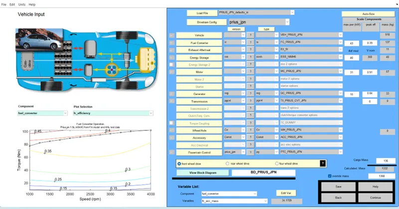
- By keeping all the parameters in the default condition, we need to continue the simulation.
- Then we need to choose the drive cycle which we want to use.
- In this experiment we choose UDDS drive cycle with 1 cycle.
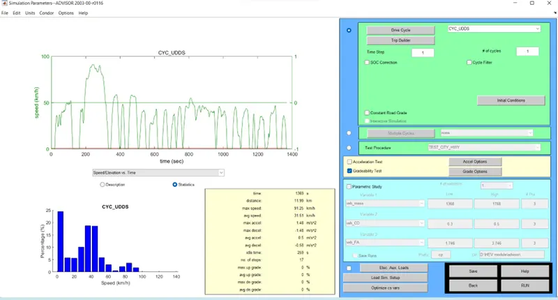
- In the same interface we will have an option called gradeability test.
- By clicking on the gradeability test option the dialog box consisting of all the test parameters for gradeability test will open.
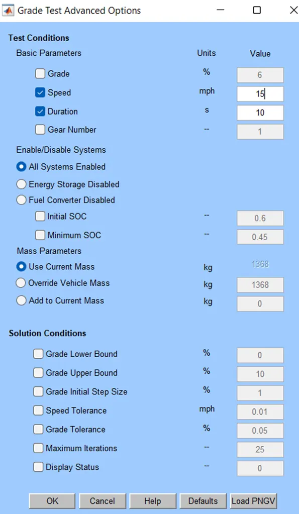
- We have done this experiment for various speeds by changing the speed during the gradeability in the gradeability test dialog box.
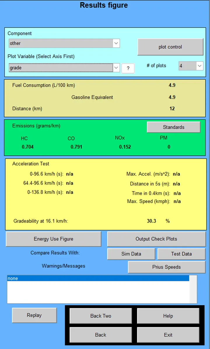
- After choosing the speed we need to run the simulation and we can observe the gradeability percentage.
Case-1 Speed 10 mph time 10sec
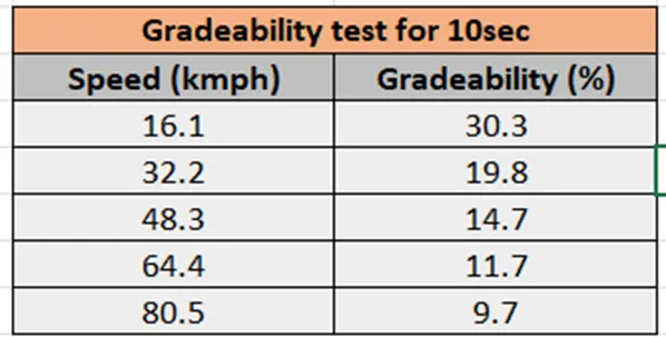
- In the case-1 we choose speed as 10 mph = 16.1 kmph and time = 10 s.
- The gradeability is 30.3% for the speed of 16.1 kmph and for a duration 10 s.
Case-2 Speed 20 mph time 10sec
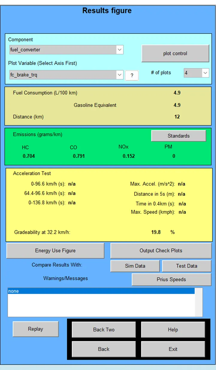
- In the case-2 we choose speed as 20 mph = 32.2 kmph and time = 10 s.
- The gradeability is 19.8% for the speed of 32.2 kmph and for a duration 10 s.
Case-3 Speed 30 mph time 10sec
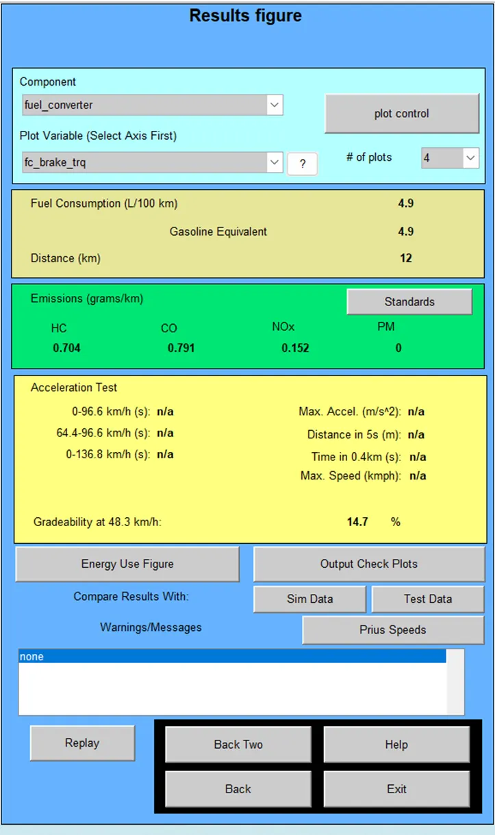
- In the case-3 we choose speed as 30 mph = 48.3 kmph and time = 10 s.
- The gradeability is 14.7% for the speed of 48.3 kmph and for a duration 10 s.
Case-4 Speed 40 mph time 10sec
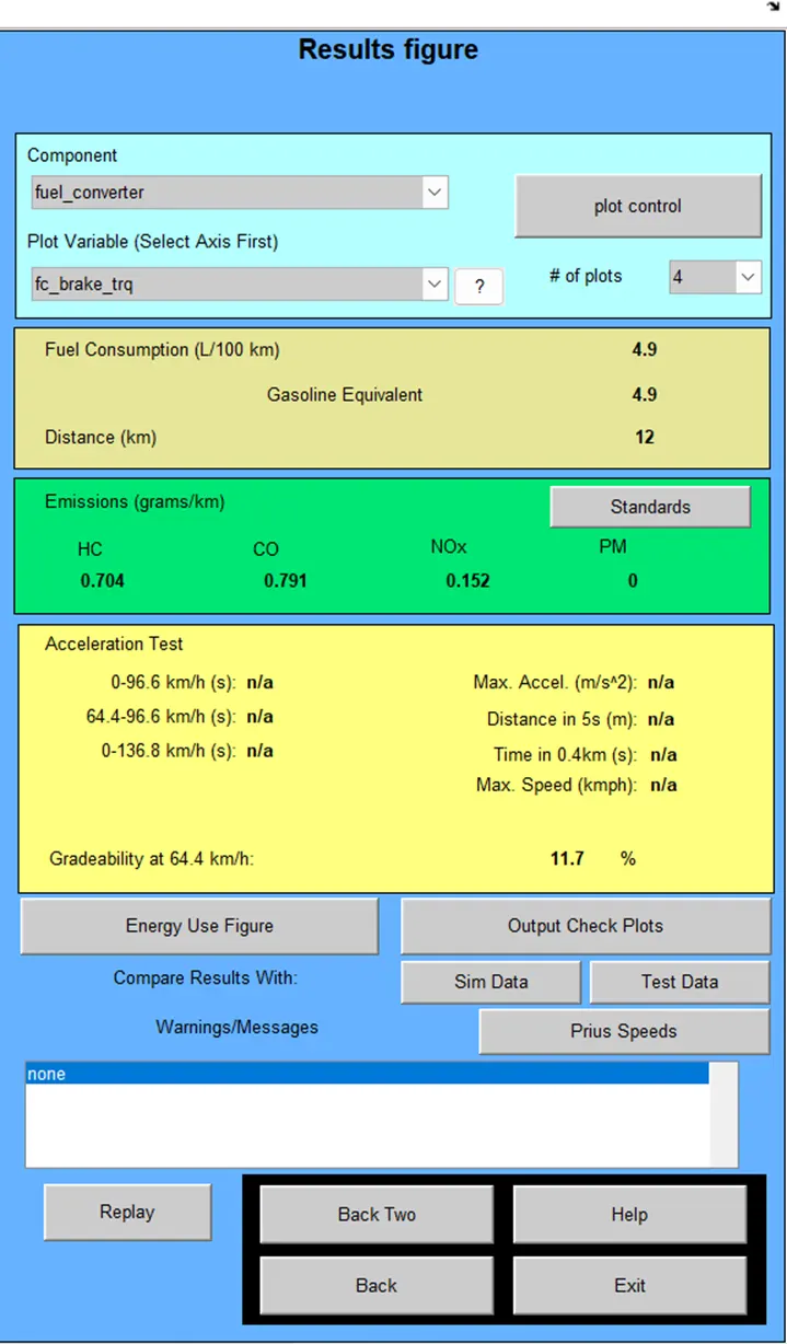
- In the case-4 we choose speed as 40 mph = 64.4 kmph and time = 10 s.
- The gradeability is 11.7% for the speed of 64.4 kmph and for a duration 10 s.
Case-5 Speed 50 mph time 10sec
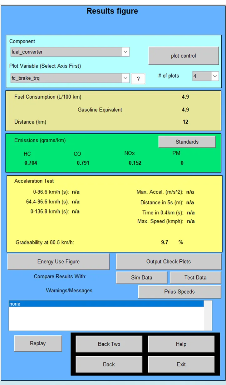
- In the case-5 we choose speed as 50 mph = 80.5 kmph and time = 10 s.
- The gradeability is 9.7% for the speed of 64.4 kmph and for a duration 10 s.
OBSERVATION:
- We can observe that for the same duration of time as the speed increases the gradeability decreases.
- The same was concluded below with the table.
CONCLUSION: