Week-3 Challenge: ADVISOR Tool

Aim : To Use the ADVISOR TOOL simulation of an electric vehicle in order to get the performance.

OBJECTIVES:

1) Initially, we are selecting EV_defaults_in file, if cargo mass is 500 kg is added with all other default conditions. We have to find can the vehicle travel for 45 km with FTP drive cycle and study the observations.

2) For the above case by changing the battery capacity we study and carry out the simulation.

3) Lastly, we are studying the gradeability test with PRIUS_Jpn_defaults_in file Compare your results.

INTRODUCTION OF ADVISOR TOOL

ADVISOR TOOL(advanced vehicle simulator model) is used to construct the models that use macro statics from duty cycles and cycle averaged efficiencis of components for near instaneneous prediction of fuel consumption and performance of the electric and hybrid vehicles. This is an old and popular tool that was created by the National Laboratary for Renewable Energy(NREL) and the development of energy in, USA. This tool uses a backward flow prorcess from the driving cycle to energy storage.

How to start the ADVISOR tool:

1. first Advisor matlab downlod.
2. To get the zip file of the advisor tool to extract the .m file.
3. Launch the MATLAB software an initially select the location of the advisor.m folder.
4. In the command window of matlab type "Advisor" and prss enter.
5. A new window will open and the select "metric" for unit and start the advisor tool. This will luanch into a new GUI called the vehicle input parameter.

ADVISOR tool consists of three windows or GUI(Graphical user interface)

• Vehicle input window.
• Simulation parameter window.
• Result window.

CASE 1:

EV_defaults_in file, if cargo mass is 500 kg is added with all other default conditions. We have to find can the vehicle travel for 45 km with FTP drive cycle.

First, select EV_defaults_in from the load file drop down menu and change parallel _default_in to EV_defaults_in from the vehicle input window

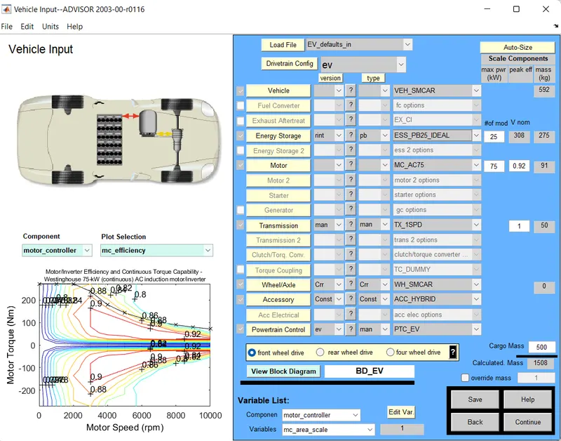
Vehicle Input Advisor Window

Now change the cargo mass to 500 Kg. By changing cargo mass total mass of the vehicle changes which can be seen.

Clicking on the continue button will be directed to the next new window which is the simulation parameter window.

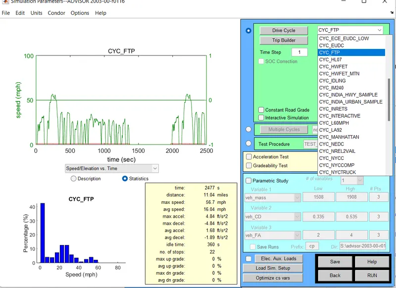
Simulation Parameter Window

In the simulation parameter window the drive cycle changes to CYC_FTP from the drive cycle drop-down menu.

Below we # of cycles for this, we have to srt the drive cycle.

After selecting the RUN button, the simulation will start and result will be displayed in a new window.

For First drive cycle

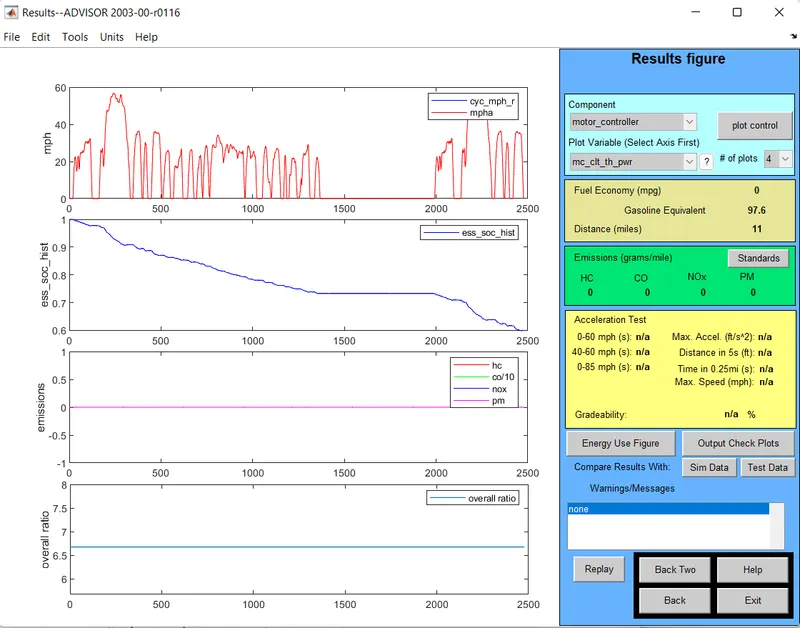
Result ADVISOR Window

The distance traveled by the vehicle in 1 drive cycle ins 11 miles(17.7 Km) where SOC is 40 % used.

Increasing the drive cycle to 2

Result-

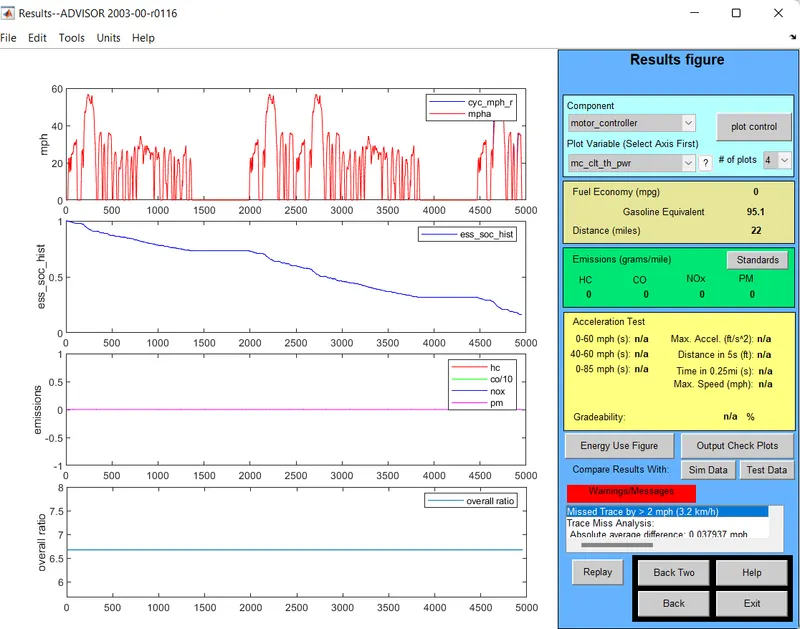
Result ADVISOR Window

The distance traveled by the vehicle in 2 drive cycle ins 22 miles(35.4 Km) where SOC is 80 % used.

Increasing drive cycle to 3

Result-

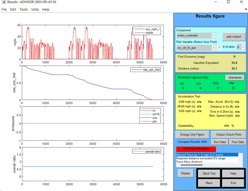
Result ADVISOR Window

The distance traveled by the vehicle in 3 drive cycle ins 25.7 miles(41.3 Km) where SOC is 100 % used.

CONCLUSION:

No. of drive cycles traveled(Km)	Distance
1	17.7
2	35.4
3	41.3

The minimum distance traveled by an electric car is 17.7 Km for the 1st drive cycle where 40% of the battery is consumed and the maximum distance traveled by an electric car is 41.3 Km which consume 100% of the battery for 3 drive cycles.

Therefore electric default cannot travel distance of 45Km due to insufficient SOC.

CASE 2:

In the above case, try changing the battery capacity and repeat the simulation.

Changing the Energy Storage to 'ESS_PB65_FocusEV' and keeping the other parameters similar to the last case.

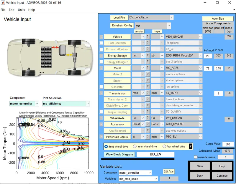
Vehicle input ADVISOR Window

Then keeping the driving cycle same we RUN the simulation.

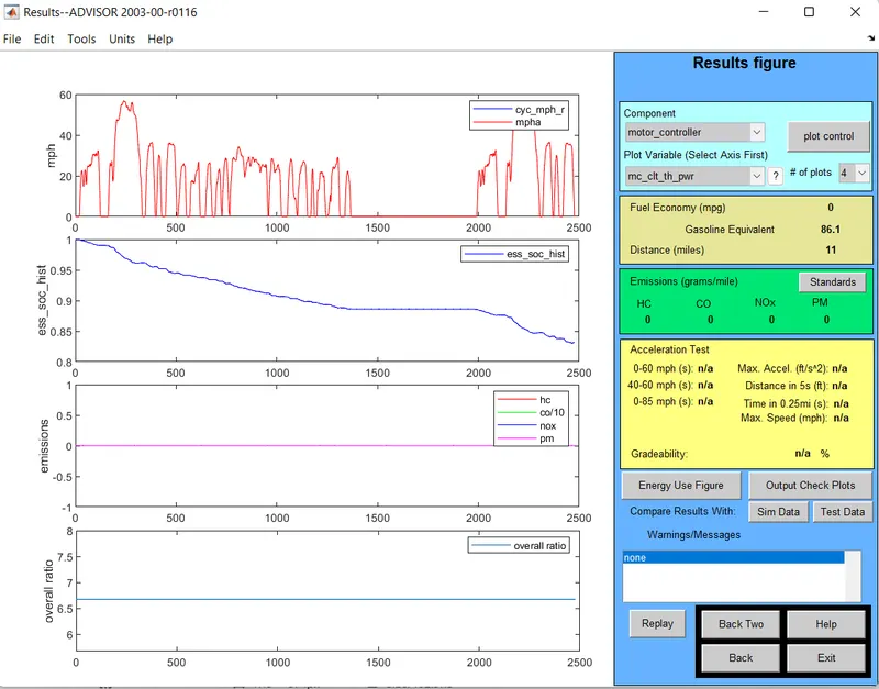
Result ADVISOR Window

From The result we can see that, Distance (Km) is 17.6 Km and the figure has not changed but, SOC % at end of 2500 seconds is 0.83 approximetly and not zero like the last case. So this means that, in one FTP cycle it covered 17.6 Km and charge is still remaining in the battery. So to get how much distance the vehicle will travelk in a single charge we need to increase the number of drive cycles for which the simulation is performed. WE will perform the simulation for 7 drive cycles.

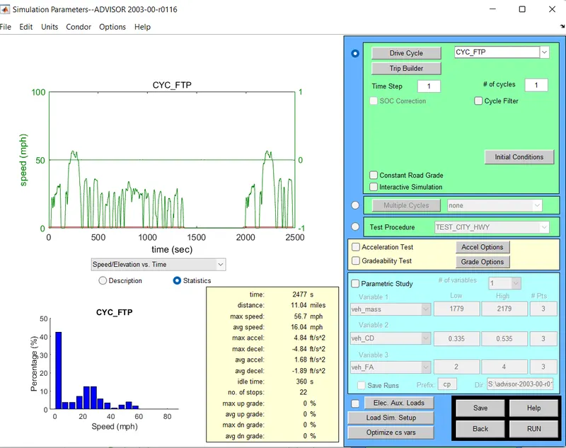
Simulation parameters ADVISOR

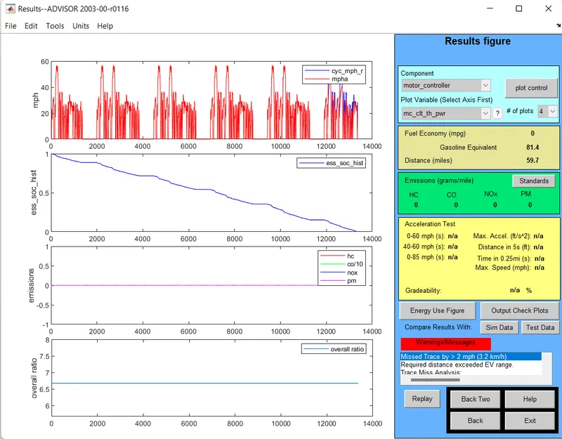
Change the value of #of cycles value to 7 from 1. Then run the simulation.

Result ADVISOR Window

From the above result we can see that, distance(Km) is 95.5 Km andalso the % of SOC as indicated by second plot is 0% by 13000 seconds approximately. So in a sigle charge the vehicle with this configuration can travel a distance of 95.5 Km in a single charge.

CASE-3

Perform the gradeability test with PRIUS_jpn_Defaults_in file. Compare your results in table and conclude.

In the load file drop down menu select 'PRIUS_jpn_Defaults_in' and rest of the parameters are kept default.

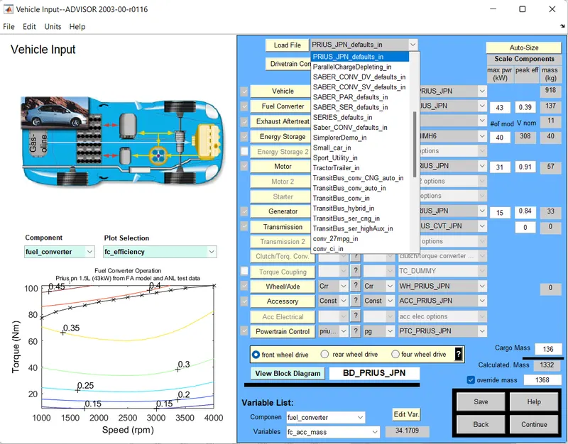
Vehicle Input ADVISOR Window

Then select continue in the bottam right corner of the window.

Select Gradeability cheakbox and then select Grade Options.

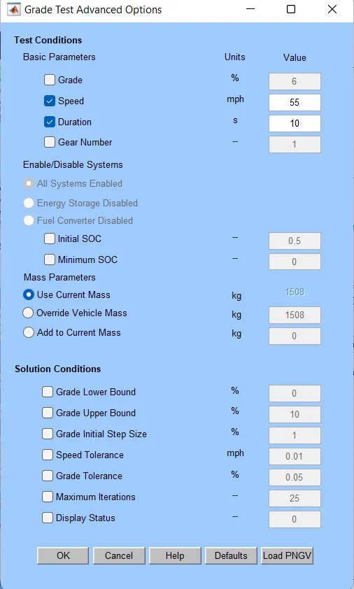
Grade Test Advance Option

The speed is kept as 55 mph.

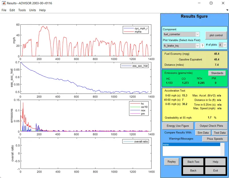
Result ADVISOR Window

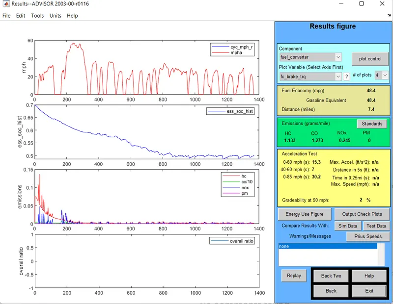
Then gadeability is 1.7%. Then speed is changed to 50.

Result ADVISOR Window

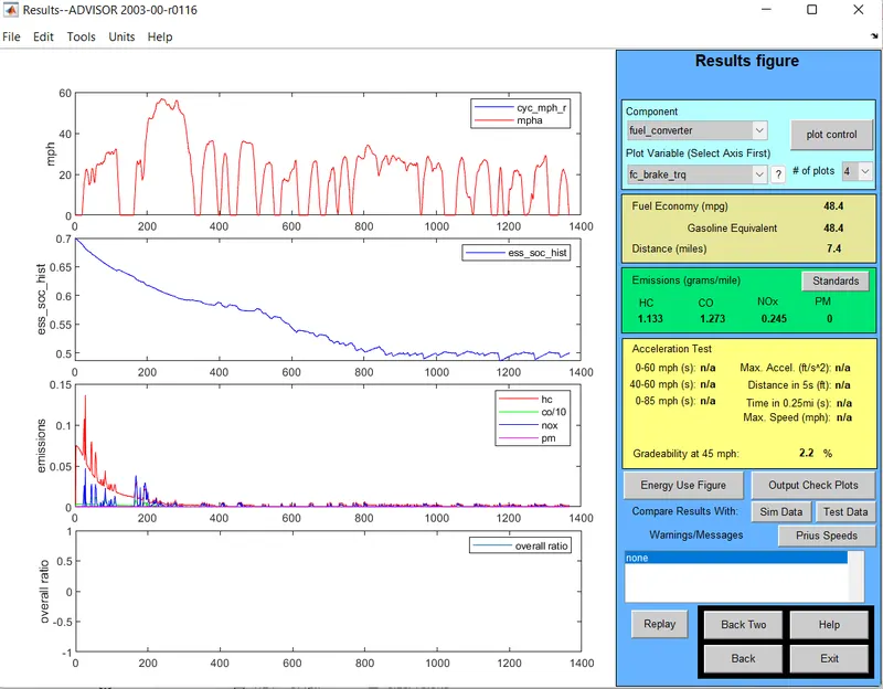
Then gradeability is 2%. Then speed is changed to 40.

Result ADVISOR Window

Then gradeability at 45 mph has increased to 2.2%.

So we can conclude by saying that, as speed increases the gradeability decreases.

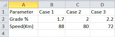
From the above table here it's seen that when the vehicle speed increases there is ecreases in gradeability for both for 10sec duration. Hence when vehicle speed increases there is a decreases gradeability.