Week 3 - Adiabatic Flame Temperature calculation
Adiabatic flame temperature variation with Equivalence ratio (In constant volume-chamber) :
Assume that methane is contained in a constant volume chamber. Write a program in Python to plot the effect of equivalence ratio on the final adiabatic flame temperature.
- Calculate the results with Cantera for varying equivalence ratios using the equilibrate method. Assume that N2 is present. Note: There are different parameters present in the equilibrate method. Use correct parameters according to type of combustion.
- Compare the results of AFT (at different equivalence ratio) for python and cantera by plotting in a single graph. Explain why AFT of both differs ?
In order to solve the following question, we need to develop the cobusiton equations with equivalence ratio as the parameter and understand the concept of Adiabatic Flame Temperature
Adiabatic Flame Temperature
The adiabatic flame temperature is the highest temperature a system can achieve at constant Pressure and also at constant volume. In the isochoric process i.e. where the volume remains constant the work done by the system wil be zero. Since we are speaking of an adiabatic process, there is no heat exchange with the surrounding as well.
A benchmark temperature for any combustion system is the “Adiabatic Flame Temperature”. It gives the essence of the maximum possible temperature rises by burning the fuel.
Here, we can define two adiabatic flame temperatures: one for constant pressure combustion and one for a constant volume
Constant Volume: In Constant-Pressure combustion, if a fuel-air mixture burns adiabatically at constant volume,
`\delta Q = \delta U + \delta W`
here U is the internal energy, W is the work done and Q is the heat delta indicates the change in the state of the system.
For a constant volume process the work done is zero and hence we can say that:
`\delta Q = \delta U`
Also as we are dealing with the adiabatic process, the change in the heat is also zero hence we can say that
`0 = \delta U`
we can finally conclude that:
`U_{Reactants}(T_{STP}, P_{STP})=U_{Products}(T, P)`
We can Know that: H =U+ PV and hence we can use this expession we obtin:
`H_{React} -P_{React}V_{React}=H_{Prod} -P_{Prod}V_{Prod}`
using the eqation of state: Pv=nRT we have
`H_{React} -H_{Prod} -P_{React}V_{React} +P_{Prod}V_{Prod}=0`
For the reactants side always the temperature is at STP unless other refrerence is specified
The final equation becomes:

constant pressure:
In Constant-Pressure combustion, if a fuel-air mixture burns adiabatically at constant pressure, the absolute enthalpy of the reactant at the initial state will be equal to the enthalpy of the products at the final state.
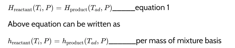
In both the approaces the adiabatic flame temperature is the solution of the equation where the variable is temperature.
Newtons Rhapsons Method:
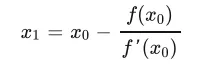
The Newton-Raphson technique is one of the most often used methods for locating roots. It is easily generalised to the issue of solving a system of nonlinear equations, which is known as Newton's approach. Furthermore, as we get closer to the root, the strategy becomes quadratically convergent. It is obtained from the taylor series expnsion of a function around a point.
The Root of the function f is found by iterating the variable x0 to x1 and so on untill the function value at the latest iteration becomes equal to zero or to a very small value called as tolerance in this case.
Equivalence ratio:
The premixing of the fuel and air prior to the flame zone creates a mixture strength that is characterized by an equivalence ratio designated by the Greek letter phi (φ). The equivalence ratio is defined as the ratio of the stoichiometric air/fuel ratio to the actual air/fuel ratio. That is
`phi =\frac {(F/A)_{Actual}} {(F/A)_{"stoichiometric"}}`
φ = 1 Stoichiometric mixture
φ < 1 Fuel lean mixture (excess air)
φ > 1 Fuel rich mixture (excess fuel)
PART-1: Effect of equivalence ratio on AFT of fuel METHANE(CH4) assuming constant volume chamber:
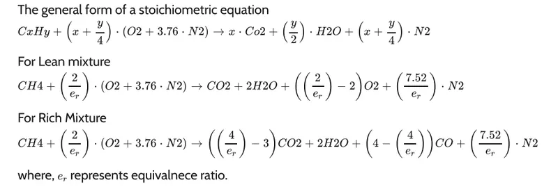
The are the equations for the combustion of methane for excess of air or exces of fuel
Structure of the python code:
- Declaring the libraries required such as numpy cantera etc
- declaring the Universal gas consta as a global variable
- decalaring the coeff used in the nasa polynomial for the evaluation of enthalpy, entropy and cp for the reactant and product species
- Writing an function file to evaluate the enthalpy of the species based on the temperature
- writing the function file to evaluate the function i.e enthalpy whose root has to be found
- writing the derivative function file which calls the function file created above and uses the delta Temp of 1e-06
- remaining portion of the code is used to write an for loop to vary the parameter of interest along with the while loop to iteratively call the function file and derivative function to use the simpsons method.
- the last part of the code is to run the cantera code to compare the results with the one made with the python code.
The code for the Adiabatic flame temperature at the cosntant volume is as shown below:
"""
	This code is written by Mr. Noble sharma as a part of the TSE CFD training to compare the variation of the Adiabatic flame temperature with the equivalence ratio
	The expression used is:
						The adiabatic flame temperature (AFT) is defined as the temperature attained when all of the chemical reaction heat released heats combustion products
						CH4+2(O2+ 3.76N2) ==> CO2+ 2H20 + 7.5 N2
						METHANE+ 2(OXYGEN + 3.76 NITROGEN)  ==> CARBON_DIOXIDE + 2 WATER + 7.5 NITROGEN
						EQUIVALENCE RATIO (PHI)=(F/A)_ACTUAL / (F/A)_STOICHIOMETRIC HERE F IS THE FUEL MOLES AND A IS THE NUMBE OF MOLES OF AIR
						PHI>1 FUEL RICH MIXTURE
						PHI=1 PROPER STOICHIOMETRIC
						PHI<1 FUEL LEAN MIXTURE
	The Equations used for describeing the combustio with rich and lean mixtures are:
						Chemical equation
						For Stiochometric ratio :: CH4 + 2 (O2 + 3.76 N2) => CO2 + 2 H2o + 7.52 N2
						For lean mixture:: CH4 + 2/eq (O2 + 3.76 N2) => CO2 + 2 H2o + (7.52/eq) N2 + (2/eq - 2) O2
						For Rich mixture:: CH4 + 2/eq (O2 + 3.76 N2) => (4/eq - 3) CO2 + 2 H2O + (7.52/eq) N2 + (4-4/eq) CO
"""
	#***************************beginning of the code ******************************************************************************************************#

	# Declaring the functions to evaluate the  actual function value, derivatives for the newton rhapsons method

	#**************************************importing key Libraries required *********************************************************
import numpy as np
import matplotlib.pyplot as plt
import math
import cantera as cant

R=8.314 #[j/ mol-K]

#Declaring the coefficients for the Equations will be used to evaluate the thermodynamic properties
CH4_coeffs_L = [5.14987613E+00, -1.36709788E-02,  4.91800599E-05, -4.84743026E-08,  1.66693956E-11, -1.02466476E+04, -4.64130376E+00]
O2_coeffs_L  = [3.78245636E+00, -2.99673416E-03,  9.84730201E-06, -9.68129509E-09,  3.24372837E-12, -1.06394356E+03,  3.65767573E+00]
O2_coeffs_H  = [3.28253784E+00,  1.48308754E-03, -7.57966669E-07,  2.09470555E-10, -2.16717794E-14, -1.08845772E+03,  5.45323129E+00]
N2_coeffs_L  = [0.03298677E+02,  0.14082404E-02, -0.03963222E-04,  0.05641515E-07, -0.02444854E-10, -0.10208999E+04,  0.03950372E+02]
N2_coeffs_H  = [0.02926640E+02,  0.14879768E-02, -0.05684760E-05,  0.10097038E-09, -0.06753351E-13, -0.09227977E+04,  0.05980528E+02]
CO2_coeffs_H = [3.85746029E+00,  4.41437026E-03, -2.21481404E-06,  5.23490188E-10, -4.72084164E-14, -4.87591660E+04,  2.27163806E+00]
H20_coeffs_H = [3.03399249E+00,  2.17691804E-03, -1.64072518E-07, -9.70419870E-11,  1.68200992E-14, -3.00042971E+04,  4.96677010E+00]
CO_coeffs_H  = [2.71518561E+00,  2.06252743E-03, -9.98825771E-07,  2.30053008E-10, -2.03647716E-14, -1.41518724E+04,  7.81868772E+00]


def Enthalpy (Temperature , coefficients):
	"""
	***Function used to caluculate the enthalpy
     H/RT = a1 + a2 T /2 + a3 T^2 /3 + a4 T^3 /4 + a5 T^4 /5 + a6/T
	"""

	a1=coefficients[0]
	a2=coefficients[1]
	a3=coefficients[2]
	a4=coefficients[3]
	a5=coefficients[4]
	a6=coefficients[5]
	a7=coefficients[6]

	h=((a1)+(a2*Temperature/2)+(a3*pow(Temperature, 2)/3)+(a4*pow(Temperature, 3)/4)+(a5*pow(Temperature, 4)/5)+(a6/Temperature))*R*Temperature

	#(a1 + a2*T/2 + a3*pow(T,2)/3 + a4*pow(T,3)/4 + a5*pow(T,4)/5 + a6/T)*R*T
	return h


def My_function( Temp, eq_Ratio):

	Temperature_STP=298.15

	# ************Calculating the enthalpy of the reactants i.e. of each species ***************************
	ENThalpy_CH4_React =Enthalpy(Temperature_STP, CH4_coeffs_L)
	ENTHALPY_O2_React  =Enthalpy(Temperature_STP, O2_coeffs_L)
	ENTHALPY_N2_React  =Enthalpy(Temperature_STP, N2_coeffs_L)

	# calculating the total enthapy:

	ENTHALPY_TOTAL_React=ENThalpy_CH4_React+(2/eq_Ratio)*(ENTHALPY_O2_React)+((2/eq_Ratio)*3.76)*ENTHALPY_N2_React  # Total enthalpy of the reactants
	NO_MOLES_React = (1)+((2/eq_Ratio))+((2/eq_Ratio)*3.76) # Number of moles of the reactants

	# ************Calculating the enthalpy of the Products i.e. of each species ***************************
	ENThalpy_CO2_Prod =Enthalpy(Temp, CO2_coeffs_H)
	ENThalpy_H2O_Prod =Enthalpy(Temp, H20_coeffs_H)
	ENThalpy_N2_Prod  =Enthalpy(Temp, N2_coeffs_H)
	ENThalpy_O2_Prod  =Enthalpy(Temp, O2_coeffs_H)
	ENThalpy_CO_Prod  =Enthalpy(Temp, CO_coeffs_H)

	# calculating the total enthapy:
	if eq_Ratio <= 1:   # Lean mixture so oxygen will also be an product

		ENTHALPY_TOTAL_Prod = (ENThalpy_CO2_Prod)+ (2*ENThalpy_H2O_Prod)+ (((2/eq_Ratio) -2)*ENThalpy_O2_Prod) + ((7.52/eq_Ratio)*ENThalpy_N2_Prod)
		NO_MOLES_Prod = (1)+(2)+((2/eq_Ratio)-2)+(7.52/eq_Ratio) # Number of moles of the product

	else:

		ENTHALPY_TOTAL_Prod = (((4/eq_Ratio) -3)*ENThalpy_CO2_Prod)+ (2*ENThalpy_H2O_Prod)+ ((-(4/eq_Ratio) +4)*ENThalpy_CO_Prod) + ((7.52/eq_Ratio)*ENThalpy_N2_Prod)
		NO_MOLES_Prod = ((4/eq_Ratio) -3)+(2)+(-(4/eq_Ratio)+4)+(7.52/eq_Ratio) # Number of moles of the produc

				#(H+nRT)_reactants - (H+nRT)_products =0
	enthalpy_func= ((ENTHALPY_TOTAL_React) - (NO_MOLES_React*R*Temperature_STP))-((ENTHALPY_TOTAL_Prod)-(NO_MOLES_Prod*R*Temp))

	return enthalpy_func


def My_function_Derivative (Temp, eq_Ratio):

	return ((My_function(Temp+1e-06, eq_Ratio)-My_function(Temp, eq_Ratio))/1e-06)

	#********************************************************Main Subroutine  begines here for Newtons Rahapsions Methosd ***************************************************


alpha=1
equivalence_ratio= np.linspace(0.2,2.0, 50)
#print("the value of the equivalence_ratio is:  n", equivalence_ratio)

Temp_array=[]

for j in equivalence_ratio:
	Temperature_guess=1500
	iteration =0
	tolerance=1e-06

	while(abs(My_function( Temperature_guess, j))>tolerance):
		Temperature_guess=Temperature_guess - alpha*(My_function(Temperature_guess, j)/My_function_Derivative(Temperature_guess, j))
		iteration=iteration+1

	Temp_array.append(Temperature_guess)
	plt.plot(j, Temperature_guess, "*", color = "red")

#print("the value of the temperature by rhapsons method is: n", Temp_array )

#************************************Code for running the cantera ***********************************************************************

import cantera as ct
#temperature array for the cantera part
T_ct = []

for j in equivalence_ratio:
# assigning gas a methane
	gas = ct.Solution("gri30.xml")
# assigning the STP value and the mole fraction for the gas
	gas.TPX = 298.15, 101325, {'CH4':1 , 'O2':2/j, 'N2':7.52/j}
# using the gas equilibrate method with constant internal energy and volume along with "auto" solver
	gas.equilibrate('UV', 'auto')
# adding the value of temperature in the array
	T_ct.append(gas.T)
# plotting the variation of temperature with change in the equivalence ratio
	plt.plot(j,gas.T,"o", color = 'blue')

print("Temperature by Cantera: n",T_ct)
# adding labels to plot
plt.xlabel("equivalence-ratio")
plt.ylabel("temperature")
plt.grid("on")
plt.show()
The plot obtained from the code is as follows:
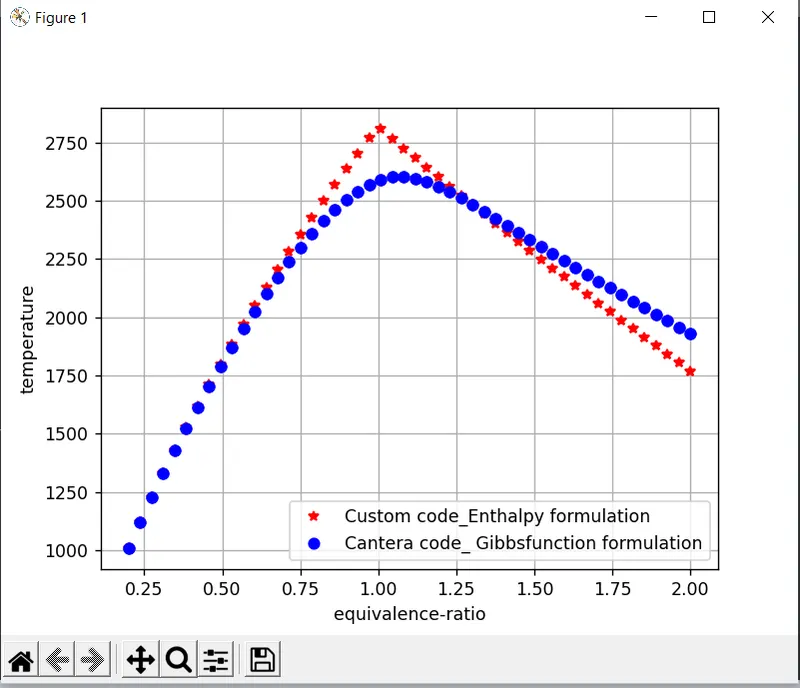
It can be observed that:
- The AFT obtained from the code and the cantera follow the same tred
- The highest AFT obtained at the EQ_ratio of 1 and after eq_ratio>1 the AFT decreases this is due to in complete combustion
- The cantera AFT is lower than the pythin code as the numbe of specied considered in the custom code are very few compared to the cantera code. Hence the heat generated is absorbed by the other species which is not accounted in our custom python code
2. Flame temperature variation with Heat loss (In constant pressure-chamber) :
- Consider a constant pressure reactor with heat loss. The reactor is initially set at STP conditions.
- The maximum heat loss for the reaction is given below. You will vary the heat loss term by multiplying the “maximum heat loss” with a factor known as H_loss_factor. Example, H_loss_factor = 0.5 would mean a heat loss for that reaction that is equal to 50% of the maximum possible heat loss.
Expected output:
- By varying the H_loss_factor from 0 to 1. Plot variation in Flame temperature w.r.t H_loss_factor
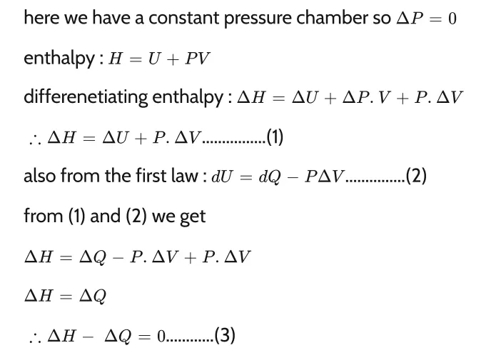
In the above Equation the DeltaQ is the loss due to non aidabatic heat condition

`H_{Prod}-H_{React}-Loss=0`
This is the function whose roots are to be found using the newton rhapsons method.
"""
	This code is written by Mr. Noble sharma as a part of the TSE CFD training to compare the variation of the Adiabatic flame temperature with the heat loss factor
	The expression used is:
						The adiabatic flame temperature (AFT) is defined as the temperature attained when all of the chemical reaction heat released heats combustion products
						CH4+2(O2+ 3.76N2) ==> CO2+ 2H20 + 7.5 N2
						METHANE+ 2(OXYGEN + 3.76 NITROGEN)  ==> CARBON_DIOXIDE + 2 WATER + 7.5 NITROGEN

 	The Equations used for describeing the combustio with rich and lean mixtures are:
						Chemical equation
						For Stiochometric ratio :: CH4 + 2 (O2 + 3.76 N2) => CO2 + 2 H2o + 7.52 N2
 """
	#***************************beginning of the code ******************************************************************************************************#

	# Declaring the functions to evaluate the  actual function value, derivatives for the newton rhapsons method

	#**************************************importing key Libraries required *********************************************************
import numpy as np
import matplotlib.pyplot as plt
import math
import cantera as cant

R=8.314 #[j/ mol-K]

#Declaring the coefficients for the Equations will be used to evaluate the thermodynamic properties
CH4_coeffs_L = [5.14987613E+00, -1.36709788E-02,  4.91800599E-05, -4.84743026E-08,  1.66693956E-11, -1.02466476E+04, -4.64130376E+00]
O2_coeffs_L  = [3.78245636E+00, -2.99673416E-03,  9.84730201E-06, -9.68129509E-09,  3.24372837E-12, -1.06394356E+03,  3.65767573E+00]
O2_coeffs_H  = [3.28253784E+00,  1.48308754E-03, -7.57966669E-07,  2.09470555E-10, -2.16717794E-14, -1.08845772E+03,  5.45323129E+00]
N2_coeffs_L  = [0.03298677E+02,  0.14082404E-02, -0.03963222E-04,  0.05641515E-07, -0.02444854E-10, -0.10208999E+04,  0.03950372E+02]
N2_coeffs_H  = [0.02926640E+02,  0.14879768E-02, -0.05684760E-05,  0.10097038E-09, -0.06753351E-13, -0.09227977E+04,  0.05980528E+02]
CO2_coeffs_H = [3.85746029E+00,  4.41437026E-03, -2.21481404E-06,  5.23490188E-10, -4.72084164E-14, -4.87591660E+04,  2.27163806E+00]
H20_coeffs_H = [3.03399249E+00,  2.17691804E-03, -1.64072518E-07, -9.70419870E-11,  1.68200992E-14, -3.00042971E+04,  4.96677010E+00]
CO_coeffs_H  = [2.71518561E+00,  2.06252743E-03, -9.98825771E-07,  2.30053008E-10, -2.03647716E-14, -1.41518724E+04,  7.81868772E+00]

def Enthalpy (Temperature , coefficients):
	"""
	***Function used to caluculate the enthalpy
     H/RT = a1 + a2 T /2 + a3 T^2 /3 + a4 T^3 /4 + a5 T^4 /5 + a6/T
	"""

	a1=coefficients[0]
	a2=coefficients[1]
	a3=coefficients[2]
	a4=coefficients[3]
	a5=coefficients[4]
	a6=coefficients[5]
	a7=coefficients[6]

	h=((a1)+(a2*Temperature/2)+(a3*pow(Temperature, 2)/3)+(a4*pow(Temperature, 3)/4)+(a5*pow(Temperature, 4)/5)+(a6/Temperature))*R*Temperature

	#(a1 + a2*T/2 + a3*pow(T,2)/3 + a4*pow(T,3)/4 + a5*pow(T,4)/5 + a6/T)*R*T
	return h


def My_function( Temp, Heat_Loss_Factor):

	Temperature_STP=298.15

	# ************Calculating the enthalpy of the reactants i.e. of each species ***************************
	ENThalpy_CH4_React =Enthalpy(Temperature_STP, CH4_coeffs_L)
	ENTHALPY_O2_React  =Enthalpy(Temperature_STP, O2_coeffs_L)
	ENTHALPY_N2_React  =Enthalpy(Temperature_STP, N2_coeffs_L)

	# calculating the total enthapy:
	eq_Ratio=1
	ENTHALPY_TOTAL_React=ENThalpy_CH4_React+(2/eq_Ratio)*(ENTHALPY_O2_React)+((2/eq_Ratio)*3.76)*ENTHALPY_N2_React  # Total enthalpy of the reactants
	NO_MOLES_React =(1)+((2/eq_Ratio))+((2/eq_Ratio)*3.76) # Number of moles of the reactants

	# ************Calculating the enthalpy of the Products i.e. of each species ***************************
	ENThalpy_CO2_Prod =Enthalpy(Temp, CO2_coeffs_H)
	ENThalpy_H2O_Prod =Enthalpy(Temp, H20_coeffs_H)
	ENThalpy_N2_Prod  =Enthalpy(Temp, N2_coeffs_H)

	ENTHALPY_TOTAL_Prod=(ENThalpy_CO2_Prod)+(2*ENThalpy_H2O_Prod)+((7.52/eq_Ratio)*ENThalpy_N2_Prod)# Total enthalpy of the reactants

	NO_MOLES_Prod =(1)+(2)+(7.52/eq_Ratio)

# Evaluating the LHV and to evalaute this we use the Enthalpies at the STP conditions only

	LHV=ENTHALPY_TOTAL_React-((Enthalpy(Temperature_STP, CO2_coeffs_H))+(2*Enthalpy(Temperature_STP, H20_coeffs_H))+(2*3.76*Enthalpy(Temperature_STP, N2_coeffs_H)))

# Evaluating the loss incurred by multiplying the LHV wth the loss fraction
	Loss=LHV*Heat_Loss_Factor

	return (ENTHALPY_TOTAL_React-ENTHALPY_TOTAL_Prod-Loss)


def My_function_Derivative (Temp, Heat_Loss_Factor):

	return ((My_function(Temp+1e-06, Heat_Loss_Factor)-My_function(Temp, Heat_Loss_Factor))/1e-06)

	#********************************************************Main Subroutine  begines here for Newtons Rahapsions Methosd ***************************************************

alpha=1
Heat_Loss_Factor=np.linspace(0,1, 100)

Temp=[]

Temp_array=[]

for j in Heat_Loss_Factor:
	Temperature_guess=1500
	iteration =0
	tolerance=1e-06

	while(abs(My_function( Temperature_guess, j))>tolerance):
		Temperature_guess=Temperature_guess - alpha*(My_function(Temperature_guess, j)/My_function_Derivative(Temperature_guess, j))
		iteration=iteration+1

	Temp_array.append(Temperature_guess)
	plt.plot(j, Temperature_guess, "--*", color = "red")

#print("the value of the temperature by rhapsons method is: n", Temp_array )

plt.xlabel("Heat-loss-factor")
plt.ylabel("temperature")
plt.grid("on")
plt.show()
plt.show()

#************************************Code for running the cantera ***********************************************************************
The output is as follows:
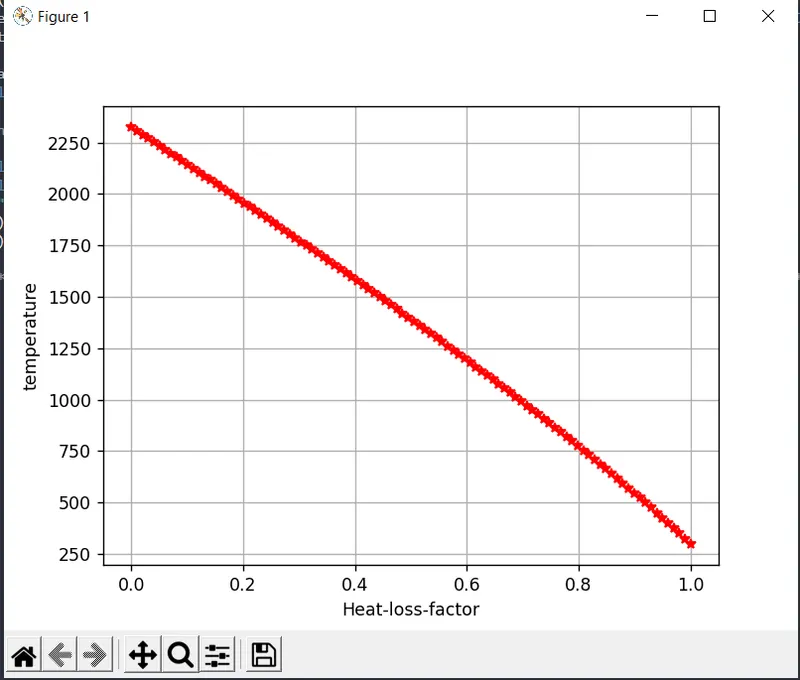
The following are the conclusions that can be made:
- The AFT decreases as the Heat loss factor is increased
-
when the heat loss factor is 0 the condition is adiabatic, so AFT will be highest
-
when the heat loss factor is 1 all the is removed from the system and we see that the temperature is less than STP condition
3. Adiabatic flame temperature variation with respect to Alkane, Alkene, Alkyne :
- Test it only for Alk -ane, -ene and -yne variants of 2 Carbon atom chains and plot a trend Assume no heat loss.
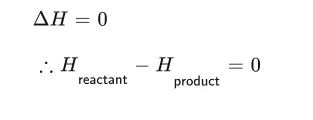
It is said that we need to run the simulation for the 2 carbon hydrocarbon with out heat loss, we can assume cosntant pressure system and hence the change in the enthalpy becomes the function whose roots are to found by rhapsons method.
The chemicial reaction equations for the combustion model are:

The code written is as follows:
"""
	This code is written by Mr. Noble sharma as a part of the TSE CFD training to compare the variation of the Adiabatic flame temperature without heat loss for alkane alkene and alkyne chanins
	The expression used is:
						The adiabatic flame temperature (AFT) is defined as the temperature attained when all of the chemical reaction heat released heats combustion products
						Alkane Reaction: C2H6 + 7/2 ( O2 + 3.76 N2) => 2 CO2 + 3 H2O + 7/2*3.76 N2
						Alkene Reaction: C2H4 + 3 (O2 + 3.76 N2) => 2 CO2 + 2 H2O + 3*3.76 N2
						Alkyne Reaction: C2H2 + 5/2 (O2 + 3.76 N2) => 2 CO2 + H2O + 5/2*3.76 N2
 	The Equations used for describeing the combustio with rich and lean mixtures are:

 	In this case the Heat loss is assumed to be zero, equivalence ratio is assumed to be 1 i.e stoichiometric combustion has taken place
  """
	#***************************beginning of the code ******************************************************************************************************#

	# Declaring the functions to evaluate the  actual function value, derivatives for the newton rhapsons method

	#**************************************importing key Libraries required *********************************************************
import numpy as np
import matplotlib.pyplot as plt
import math
import cantera as cant

R=8.314 #[j/ mol-K]

#Declaring the coefficients for the Equations will be used to evaluate the thermodynamic properties


C2H6_coeffs_L= [4.29142492E+00, -5.50154270E-03,  5.99438288E-05, -7.08466285E-08,  2.68685771E-11, -1.15222055E+04,  2.66682316E+00]
C2H4_coeffs_L= [3.95920148E+00, -7.57052247E-03,  5.70990292E-05, -6.91588753E-08,  2.69884373E-11,  5.08977593E+03,  4.09733096E+00]
C2H2_coeffs_L= [8.08681094E-01,  2.33615629E-02, -3.55171815E-05,  2.80152437E-08, -8.50072974E-12,  2.64289807E+04,  1.39397051E+01]
CH4_coeffs_L = [5.14987613E+00, -1.36709788E-02,  4.91800599E-05, -4.84743026E-08,  1.66693956E-11, -1.02466476E+04, -4.64130376E+00]
O2_coeffs_L  = [3.78245636E+00, -2.99673416E-03,  9.84730201E-06, -9.68129509E-09,  3.24372837E-12, -1.06394356E+03,  3.65767573E+00]
O2_coeffs_H  = [3.28253784E+00,  1.48308754E-03, -7.57966669E-07,  2.09470555E-10, -2.16717794E-14, -1.08845772E+03,  5.45323129E+00]
N2_coeffs_L  = [0.03298677E+02,  0.14082404E-02, -0.03963222E-04,  0.05641515E-07, -0.02444854E-10, -0.10208999E+04,  0.03950372E+02]
N2_coeffs_H  = [0.02926640E+02,  0.14879768E-02, -0.05684760E-05,  0.10097038E-09, -0.06753351E-13, -0.09227977E+04,  0.05980528E+02]
CO2_coeffs_H = [3.85746029E+00,  4.41437026E-03, -2.21481404E-06,  5.23490188E-10, -4.72084164E-14, -4.87591660E+04,  2.27163806E+00]
H20_coeffs_H = [3.03399249E+00,  2.17691804E-03, -1.64072518E-07, -9.70419870E-11,  1.68200992E-14, -3.00042971E+04,  4.96677010E+00]
CO_coeffs_H  = [2.71518561E+00,  2.06252743E-03, -9.98825771E-07,  2.30053008E-10, -2.03647716E-14, -1.41518724E+04,  7.81868772E+00]

def Enthalpy (Temperature , coefficients):
	"""
	***Function used to caluculate the enthalpy
     H/RT = a1 + a2 T /2 + a3 T^2 /3 + a4 T^3 /4 + a5 T^4 /5 + a6/T
	"""

	a1=coefficients[0]
	a2=coefficients[1]
	a3=coefficients[2]
	a4=coefficients[3]
	a5=coefficients[4]
	a6=coefficients[5]
	a7=coefficients[6]

	h=((a1)+(a2*Temperature/2)+(a3*pow(Temperature, 2)/3)+(a4*pow(Temperature, 3)/4)+(a5*pow(Temperature, 4)/5)+(a6/Temperature))*R*Temperature

	#(a1 + a2*T/2 + a3*pow(T,2)/3 + a4*pow(T,3)/4 + a5*pow(T,4)/5 + a6/T)*R*T
	return h


def My_function( Temp, No_Bonds):

	Temperature_STP=298.15

	# ************Calculating the enthalpy of the reactants i.e. of each species ***************************


	ENThalpy_C2H6_React =Enthalpy(Temperature_STP, C2H6_coeffs_L)
	ENThalpy_C2H4_React =Enthalpy(Temperature_STP, C2H4_coeffs_L)
	ENThalpy_C2H2_React =Enthalpy(Temperature_STP, C2H2_coeffs_L)

	ENThalpy_CH4_React  =Enthalpy(Temperature_STP, CH4_coeffs_L)
	ENTHALPY_O2_React   =Enthalpy(Temperature_STP, O2_coeffs_L)
	ENTHALPY_N2_React   =Enthalpy(Temperature_STP, N2_coeffs_L)

	# calculating the total enthapy:
	eq_Ratio=1
#	ENTHALPY_TOTAL_React=ENThalpy_CH4_React+(2/eq_Ratio)*(ENTHALPY_O2_React)+((2/eq_Ratio)*3.76)*ENTHALPY_N2_React  # Total enthalpy of the reactants
#	NO_MOLES_React =(1)+((2/eq_Ratio))+((2/eq_Ratio)*3.76) # Number of moles of the reactants

	# ************Calculating the enthalpy of the Products i.e. of each species ***************************
	ENThalpy_CO2_Prod =Enthalpy(Temp, CO2_coeffs_H)
	ENThalpy_H2O_Prod =Enthalpy(Temp, H20_coeffs_H)
	ENThalpy_N2_Prod  =Enthalpy(Temp, N2_coeffs_H)

#	ENTHALPY_TOTAL_Prod=(ENThalpy_CO2_Prod)+(2*ENThalpy_H2O_Prod)+((7.52/eq_Ratio)*ENThalpy_N2_Prod)# Total enthalpy of the reactants

#	NO_MOLES_Prod =(1)+(2)+(7.52/eq_Ratio)

	if No_Bonds==1: # Alkanes i.e. C-C bound is one only

		ENTHALPY_TOTAL_React = ENThalpy_C2H6_React + 7/2*(ENTHALPY_O2_React + 3.76*ENTHALPY_N2_React)
		ENTHALPY_TOTAL_Prod = 2*ENThalpy_CO2_Prod + 3*ENThalpy_H2O_Prod + 7/2*3.76*ENThalpy_N2_Prod

	elif No_Bonds==2: # Alkene i.e. C-C bound is two

		ENTHALPY_TOTAL_React = ENThalpy_C2H4_React + 3*(ENTHALPY_O2_React + 3.76*ENTHALPY_N2_React)
		ENTHALPY_TOTAL_Prod = 2*ENThalpy_CO2_Prod + 2*ENThalpy_H2O_Prod + 3*3.76*ENThalpy_N2_Prod

	else:
		ENTHALPY_TOTAL_React = ENThalpy_C2H2_React + 5/2*(ENTHALPY_O2_React + 3.76*ENTHALPY_N2_React)
		ENTHALPY_TOTAL_Prod = 2*ENThalpy_CO2_Prod + ENThalpy_H2O_Prod + (5/2)*3.76*ENThalpy_N2_Prod


	return ENTHALPY_TOTAL_Prod - ENTHALPY_TOTAL_React


def My_function_Derivative (Temp, No_Bonds):

	return ((My_function(Temp+1e-06, No_Bonds)-My_function(Temp, No_Bonds))/1e-06)

	#********************************************************Main Subroutine  begines here for Newtons Rahapsions Methosd ***************************************************

alpha=0.5
tolerance=1e-06
n_bonds=[1,2,3]
Temp_array=[]

for j in n_bonds:
	Temperature_guess=1500
	iteration =0

	while(abs(My_function( Temperature_guess, j))>tolerance):
		Temperature_guess=Temperature_guess - alpha*(My_function(Temperature_guess, j)/My_function_Derivative(Temperature_guess, j))
		iteration=iteration+1

	Temp_array.append(Temperature_guess)

#print("the value of the temperature by rhapsons method is: n", Temp_array )


#************************************Code for running the cantera ***********************************************************************

gas = cant.Solution('gri30.xml')
gas.TPX = 298.15,101325,{'C2H6':1,'O2':3.5,'N2':3.5*3.76}
gas.equilibrate('HP','auto')
T_alkane = gas.T
gas.TPX = 298.15,101325,{'C2H4':1,'O2':3,'N2':3*3.76}
gas.equilibrate('HP','auto')
T_alkene = gas.T
gas.TPX = 298.15,101325,{'C2H2':1,'O2':2.5,'N2':2.5*3.76}
gas.equilibrate('HP','auto')

T_alkyne = gas.T

T = (T_alkane,T_alkene,T_alkyne)
T= np.array(T)


plt.figure(1)
plt.plot(n_bonds, Temp_array,"*", color = "red" , label='Custom code_Enthalpy formulation', ls='-')
plt.plot(n_bonds, T,"o", color = "blue" , label='Cantera code', ls='-')
plt.legend()
plt.xlabel("number of carbon bonds")
plt.ylabel("AFT")
plt.grid("on")
plt.show()
plt.line
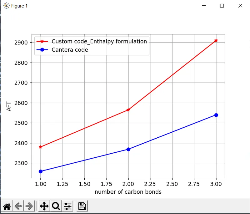
It can be seen that:
- as the number of carbon bonds increases the AFT is also higher as the energy required to break the triple bond>double bond>singlebond
- The prediction by cantera is on lower side compared to the custom code as stated in the previous section
4. Adiabatic flame temperature variation with respect to number of Carbon atom chains :
The following equations are used to run the simulaiton:

Here the input is the number 1 2 3 and all the remaining things are evalated automatically in the function file:
The code is as follows:
"""
	This code is written by Mr. Noble sharma as a part of the TSE CFD training to compare the variation of the Adiabatic flame temperature without heat loss for Methane, Ethane and Propane
	The expression used is: The adiabatic flame temperature (AFT) is defined as the temperature attained when all of the chemical reaction heat released heats combustion productsAlkyne Reaction: C2H2 + 5/2 (O2 + 3.76 N2) => 2 CO2 + H2O + 5/2*3.76 N2
 	Chemical equations:
		General representation of stoichiometric reaction written as
						CxHy + (x+y/4)*(O2+3.76*N2) -> x*Co2 + (y/2)*H2O + (x+y/4)*3.76*N2
 							(Reactants) -> (Products)
						C1
						CH4 + 2 (O2 + 3.76 N2) => CO2 + 2 H2o + 7.52 N2
						C2
						C2H6 + 7/2 ( O2 + 3.76 N2 ) => 2 CO2 + 3 H2O + 7/2*3.76 N2
						C3
						C3H8 + 5 (O2 + 3.76 N2) => 3 CO2 + 4 H2O + 5*3.76 N2


 	The Equations used for describeing the combustio with rich and lean mixtures are:

 	In this case the Heat loss is assumed to be zero, equivalence ratio is assumed to be 1 i.e stoichiometric combustion has taken place
  """
	#***************************beginning of the code ******************************************************************************************************#

	# Declaring the functions to evaluate the  actual function value, derivatives for the newton rhapsons method

	#**************************************importing key Libraries required *********************************************************
import numpy as np
import matplotlib.pyplot as plt
import math
import cantera as cant

R=8.314 #[j/ mol-K]

#Declaring the coefficients for the Equations will be used to evaluate the thermodynamic properties
CH4_coeffs_L = [5.14987613E+00, -1.36709788E-02,  4.91800599E-05, -4.84743026E-08,  1.66693956E-11, -1.02466476E+04, -4.64130376E+00]
C2H6_coeffs_L= [4.29142492E+00, -5.50154270E-03,  5.99438288E-05, -7.08466285E-08,  2.68685771E-11, -1.15222055E+04,  2.66682316E+00]
C3H8_coeffs_L =[0.93355381E+00,  0.26424579E-01,  0.61059727E-05,  -0.21977499E-07, 0.95149253E-11, -0.13958520E+05,  0.19201691E+02]
O2_coeffs_L  = [3.78245636E+00, -2.99673416E-03,  9.84730201E-06, -9.68129509E-09,  3.24372837E-12, -1.06394356E+03,  3.65767573E+00]
O2_coeffs_H  = [3.28253784E+00,  1.48308754E-03, -7.57966669E-07,  2.09470555E-10, -2.16717794E-14, -1.08845772E+03,  5.45323129E+00]
N2_coeffs_L  = [0.03298677E+02,  0.14082404E-02, -0.03963222E-04,  0.05641515E-07, -0.02444854E-10, -0.10208999E+04,  0.03950372E+02]
N2_coeffs_H  = [0.02926640E+02,  0.14879768E-02, -0.05684760E-05,  0.10097038E-09, -0.06753351E-13, -0.09227977E+04,  0.05980528E+02]
CO2_coeffs_H = [3.85746029E+00,  4.41437026E-03, -2.21481404E-06,  5.23490188E-10, -4.72084164E-14, -4.87591660E+04,  2.27163806E+00]
H20_coeffs_H = [3.03399249E+00,  2.17691804E-03, -1.64072518E-07, -9.70419870E-11,  1.68200992E-14, -3.00042971E+04,  4.96677010E+00]
CO_coeffs_H  = [2.71518561E+00,  2.06252743E-03, -9.98825771E-07,  2.30053008E-10, -2.03647716E-14, -1.41518724E+04,  7.81868772E+00]

def Enthalpy (Temperature , coefficients):
	"""
	***Function used to caluculate the enthalpy
     H/RT = a1 + a2 T /2 + a3 T^2 /3 + a4 T^3 /4 + a5 T^4 /5 + a6/T
	"""

	a1=coefficients[0]
	a2=coefficients[1]
	a3=coefficients[2]
	a4=coefficients[3]
	a5=coefficients[4]
	a6=coefficients[5]
	a7=coefficients[6]

	h=((a1)+(a2*Temperature/2)+(a3*pow(Temperature, 2)/3)+(a4*pow(Temperature, 3)/4)+(a5*pow(Temperature, 4)/5)+(a6/Temperature))*R*Temperature

	#(a1 + a2*T/2 + a3*pow(T,2)/3 + a4*pow(T,3)/4 + a5*pow(T,4)/5 + a6/T)*R*T
	return h


def My_function( Temp, No_Carbons):

	Temperature_STP=298.15

	# ************Calculating the enthalpy of the reactants i.e. of each species ***************************

	ENTHALPY_O2_React   =Enthalpy(Temperature_STP, O2_coeffs_L)
	ENTHALPY_N2_React   =Enthalpy(Temperature_STP, N2_coeffs_L)

	# calculating the total enthapy:
	eq_Ratio=1

	# ************Calculating the enthalpy of the Products i.e. of each species ***************************
	ENThalpy_CO2_Prod =Enthalpy(Temp, CO2_coeffs_H)
	ENThalpy_H2O_Prod =Enthalpy(Temp, H20_coeffs_H)
	ENThalpy_N2_Prod  =Enthalpy(Temp, N2_coeffs_H)

#	ENTHALPY_TOTAL_Prod=(ENThalpy_CO2_Prod)+(2*ENThalpy_H2O_Prod)+((7.52/eq_Ratio)*ENThalpy_N2_Prod)# Total enthalpy of the reactants

#	NO_MOLES_Prod =(1)+(2)+(7.52/eq_Ratio)

	if No_Carbons==1: # Alkanes i.e. C-C bound is one only

		ENThalpy_CH4_React  =Enthalpy(Temperature_STP, CH4_coeffs_L)
		x = 1
		y = 2*(x+1)
		a = x + y/4
		b = y/2
		ENTHALPY_TOTAL_React = ENThalpy_CH4_React + a*ENTHALPY_O2_React + 3.76*a*ENTHALPY_N2_React # Enthalpy in J basis
		ENTHALPY_TOTAL_Prod = x*ENThalpy_CO2_Prod + b*ENThalpy_H2O_Prod + 3.76*a*ENThalpy_N2_Prod # Enthalpy in J basis

	elif No_Carbons==2: # Alkene i.e. C-C bound is two

		ENThalpy_C2H6_React =Enthalpy(Temperature_STP, C2H6_coeffs_L)
		x = 2
		y = 2*(x+1)
		a = x + y/4
		b = y/2

		ENTHALPY_TOTAL_React = ENThalpy_C2H6_React + a*ENTHALPY_O2_React + 3.76*a*ENTHALPY_N2_React # Enthalpy in J basis
		ENTHALPY_TOTAL_Prod = x*ENThalpy_CO2_Prod + b*ENThalpy_H2O_Prod + 3.76*a*ENThalpy_N2_Prod # Enthalpy in J basis


	else:

		ENThalpy_C3H8_React =Enthalpy(Temperature_STP, C3H8_coeffs_L)
		x = 3
		y = 2*(x+1)
		a = x + y/4
		b = y/2

		ENTHALPY_TOTAL_React = ENThalpy_C3H8_React + a*ENTHALPY_O2_React + 3.76*a*ENTHALPY_N2_React # Enthalpy in J basis
		ENTHALPY_TOTAL_Prod = x*ENThalpy_CO2_Prod + b*ENThalpy_H2O_Prod + 3.76*a*ENThalpy_N2_Prod # Enthalpy in J basis

	return ENTHALPY_TOTAL_Prod - ENTHALPY_TOTAL_React


def My_function_Derivative (Temp, No_Carbons):

	return ((My_function(Temp+1e-06, No_Carbons)-My_function(Temp, No_Carbons))/1e-06)

alpha=0.5
tolerance=1e-06
No_Carbons=[1,2,3]
Temp_array=[]

for j in No_Carbons:
	Temperature_guess=1500
	iteration =0

	while(abs(My_function( Temperature_guess, j))>tolerance):
		Temperature_guess=Temperature_guess - alpha*(My_function(Temperature_guess, j)/My_function_Derivative(Temperature_guess, j))
		iteration=iteration+1

	Temp_array.append(Temperature_guess)


plt.figure(1)
plt.plot(No_Carbons,Temp_array  , ls= "--", color = "red")
plt.xlabel("number of carbon atoms")
plt.ylabel("AFT")
plt.grid("on")
 #print("the value of the temperature by rhapsons method is: n", Temp_array )
plt.show()
The output obtained is as follows:
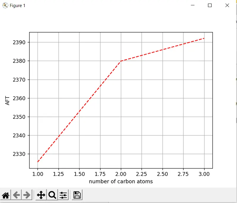
it can be seen that:
we can see as the number of carbon atom increases the AFT values also increases but the growth in temperature values is non linear. This can be attributed to the fact that propane has three c atoms and hence releases highest amount of heat and the AFT will be higher.