Challenge

Week 3 - Adiabatic Flame Temperature calculation

VVikas Rai1 Feb 2022

AIM: Adiabatic Flame Temperature Calculation for different cases using Python and Cantera.

OBJECTIVE:

1. Adiabatic Flame Temperature variation with Equivalence ratio (In constant volume-chamber):

Write a program in Python to plot the effect of equivalence ratio on the final adiabatic flame temperature. Assume that methane is contained in a constant volume chamber.
Calculate the results with Cantera for varying equivalence ratios using the equilibrate method. Assume that N2 is present.
Compare the results of AFT (at different equivalence ratios) for Python and Cantera by plotting in a single graph. Explain why the AFT of both differs.

2. Flame temperature variation with Heat loss (In constant pressure-chamber):

Consider a constant pressure reactor with heat loss. The reactor is initially set at STP conditions.
By varying the H_loss_factor from 0 to 1. Plot variation in Flame Temperature w.r.t. H_loss_factor.

3. Adiabatic flame temperature variation with respect to Alkane, Alkene, Alkyne:

Test it only for Alk -ane, -ene, and -yne variants of 2 Carbon atom chains and plot a trend Assume no heat loss.

4. Adiabatic flame temperature variation with respect to the number of Carbon atom chains:

For a general alkane, plot the effect of the number of Carbon atoms (from 1 to 3) on the final temperature. Assume no heat loss.

THEORY:

Enthalpy:

The heat energy, which is evolved or absorbed during a chemical reaction progression, is called enthalpy. It is represented by H, and the letter H indicates the energy amount. Enthalpy change is given by `DeltaH`where the delta symbol shows the change and its unit is joules or kilojoules.

It can be said that sum of internal energies of the system is enthalpy. The reason is that a change in internal energy takes place at the time of chemical reaction, and this change is calculated as enthalpy. It can be given by the following expression:

`H = U + PV`

Where H = enthalpy,

U = sum of internal energy,

P = pressure of system,

V = volume of system.

So, enthalpy is the addition of internal energy and energy needed to conserve a system's volume at a given pressure. PV represents the work that is required to be done on the environment to create space for the system.

Internal Energy:

A system's internal energy refers to the addition of the potential and kinetic energy of that particular system. The stored energy is potential energy and the energy released due to the movement of molecules is kinetic energy. Moreover, the internal energy is represented by U, and the change in internal energy is given by `DeltaU`.

At constant pressure, internal energy and enthalpy are the same for a particular system. Internal energy change can take place in two ways. One is because of the transfer of heat - a system can absorb or release heat, and the second is by doing work. Hence, internal energy change can be expressed by the following equation:

`DeltaU = q + w`

Where `DeltaU =` internal energy change,

q = transfer of heat,

w = work done by or on a system.

Adiabatic Flame Temperature:

The adiabatic flame temperature (AFT) is defined as the temperature attained when all of the chemical reaction heat released heats combustion products. The adiabatic flame temperature is the maximum temperature of the combustion gas that can be reached by the combustion reaction under no heat loss to the surroundings in the adiabatic condition. In other words, In a combustion process, the final temperature attained under adiabatic conditions is known as adiabatic flame temperature (`T_(ad)`).

The adiabatic flame temperature depends on initial pressure, initial temperature, reactant composition.

Significance:

It is used to characterize the quality of the fuel.
It is used to determine the suitability of fuel for an application.
It is used to determine the extent of substitution of lower quality fuel to converse higher quality fuel.
It is very important in the design and scale-up procedures wherever heat transfer is a significant consideration.

In the study of combustion, there are two types of adiabatic flame temperature depending on how the process is completed: the constant volume and constant pressure.

The constant volume adiabatic flame temperature is the temperature that results from a complete combustion process that occurs without any work, heat transfer or changes in kinetic or potential energy. This is the maximum temperature that can be achieved for given reactants because any heat transfer from the reacting substances and/or any incomplete combustion would tend to lower the temperature of the products.

Enthalpy equation for constant volume combustion

Using the enthalpy definition we can write

`H = U + PV`

We can modify the equation for change in it

`DeltaH = DeltaU + Delta(PV)`

Now, if we assume volume is constant, then we can take the V out to get

`DeltaH = DeltaU + VDeltaP`

We have from the first law of thermodynamics,

`DeltaU = q + W`

For a constant volume process, there is no work done by the system due to no change in the volume. Hence, the heat generated q is completely used in increasing the internal energy U of the system, so we can write as

`DeltaU = q`

Therefore, `DeltaH = q + VDeltaP`

For an adiabatic process, q = 0

Therefore, `DeltaH - VDeltaP= 0`

We can write the above equation in the following form for our case,

`H_(Product) - H_(Reactant) - V(P_(Initial) - P_(f)) = 0`

According to ideal gas relation PV = nRT

`P_(Initial).V = N_(reactants).R.T_(Initial)`

`P_(f).V = N_(Products).R.T_(ad)`

Thus equation can be written as,

`H_(Product) - H_(Reactant) - R.(N_(Product).T_(ad) - N_(Reactant).T_(Initial)) = 0`

The constant pressure adiabatic flame temperature is the temperature that results from a complete combustion process that occurs without ant heat transfer or changes in kinetic or potential energy. Its temperature is lower than the constant volume process because some of the energy is utilized to change the volume of the system (i.e., generate work).

Enthalpy equation for constant pressure combustion

Using the enthalpy definition we can write

`H = U + PV`

We can modify the equation for change in it

`DeltaH = DeltaU + Delta(PV)`

Now, if we assume the pressure is constant, then we can take the P out to get

`DeltaH = DeltaU + PDeltaV`

Now PV work (or the expansion work) is defined as `W = -PDeltaV`, so we have from the first law of thermodynamics (`DeltaU = q + W`),

`DeltaU = q - PDeltaV`

Therefore at constant pressure, we have

`DeltaH = q - PDeltaV + PDeltaV`

`DeltaH = q`

Under adiabatic condition, q = 0,

therfore, `DeltaH = 0`

`H_(Product) = H_(Reactant)`

`H_(Product) - H_(Reactant) = 0`

SOLVING APPROACH:

Here the enthalpy of the products and reactants are calculated by using the NASA polynomial function.

`H = (a_1 + a_2(T/2) + a_3(T^2/3) + a_4(T^3/4) + a_5(T^4/5) + a_6/T)*R*T`

where `a_1,a_2,a_3,a_4,a_5,a_6 and a_7` are the numerical coefficients supplied in NASA thermodynamics files (http://combustion.berkeley.edu/gri_mech/version30/files30/thermo30.dat).

T = temperature

R = gas constant

Then Newton Raphson method is used to solve the enthalpy. Using this method we will find out the roots of the function using the initial guess and iterate till we reach the given tolerance value. It is defined as

`T_(New) = T_(guess) - alpha[(f(T_(guess)))/(f'(T_(guess)))]`

where `T_(New)` = New T value after iteration

`T_(guess)` = guessed T value

`alpha` = relaxation factor

SOLUTION:

CASE 1. Adiabatic Flame Temperature variation with Equivalence ratio (In constant volume-chamber)

The stoichiometric quantity of oxidizer is just that amount needed to completely burn a quantity of fuel. If more than a stoichiometric quantity of oxidizer is supplied, the mixture is said to fuel lean, or just lean; while supplying less than the stoichiometric oxidizer results in a fuel-rich, or rich mixture.

The equivalence ratio, `phi`, is commonly used to indicate quantitatively whether a fuel-oxidizer mixture is rich, lean, or stoichiometric. The equivalence ratio is defined as

`phi = ((A/F)_(stOich))/((A/F)) = ((F/A))/((F/A)_(stOich))`

From this definition, we see that for fuel-rich mixtures, `phi>1`, and for fuel-lean mixtures, `phi<1`. For a stoichiometric mixture, `phi` equals unity.

For `phi = 1`, The stoichiometric mixture of combustion of methane looks like the following:

`CH_4 + 2*(O_2+3.76*N_2) -> CO_2 + 2*H_(2)O + 7.52*N_2`

For `phi <1`(lean mixture):

`CH_4 + (2/phi)*(O_2+3.76*N_2) -> CO_2 + 2H_(2)O + ((2/phi)-2)*O_2 + (7.52/phi)*N_2`

For `phi >1`(rich mixture):

`CH_4 + (2/phi)*(O2+3.76*N_2) -> ((4/phi)-3)*CO_2 + 2H_(2)O + (4-(4/phi))*CO + (7.52/phi)*N_2`

CODE: Python and Cantera Code to calculate Adiabatic Flame Temperature variation with Equivalence ratio (In constant volume-chamber):

"""
Programm to find out the effect of equivalence ratio on AFT in constant volume chamber

For stoichiometric mixture
CH4 + 2*(O2+3.76*N2) -> CO2 + 2*H2O + 7.52*N2

For Lean Mixture
CH4 + (2/e_r)*(O2+3.76*N2) -> CO2 + 2H2O + ((2/e_r)-2)*O2 + (7.52/e_r)*N2

For Reach Mixture
CH4 + (2/e_r)*(O2+3.76*N2) -> ((4/e_r)-3)*CO2 + 2H2O + (4-(4/e_r))*CO + (7.52/e_r)*N2
"""

import matplotlib.pyplot as plt
import numpy

# Equivalence ratio
e_r = numpy.linspace(0.1,2.0,20)


# Function to evaluate enthalpy
def h(T,co_effs):
	
	R = 8.314 # J/mol-K	
	a1 = co_effs[0]
	a2 = co_effs[1]
	a3 = co_effs[2]
	a4 = co_effs[3]
	a5 = co_effs[4]
	a6 = co_effs[5]
	return (a1 + a2*T/2 + a3*pow(T,2)/3 + a4*pow(T,3)/4 +  a5*pow(T,4)/5 + a6/T)*R*T

# Low temperature coefficients (Reactants) at STP condition
CH4_coeffs_l = [5.14987613E+00,-1.36709788E-02,4.91800599E-05,-4.84743026E-08,1.66693956E-11,-1.02466476E+04,-4.64130376E+00]
O2_coeffs_l = [3.78245636E+00,-2.99673416E-03,9.84730201E-06,-9.68129509E-09,3.24372837E-12,-1.06394356E+03,3.65767573E+00]
N2_coeffs_l = [0.03298677E+02,0.14082404E-02,-0.03963222E-04,0.05641515E-07,-0.02444854E-10,-0.10208999E+04,0.03950372E+02]

# High-temperature coefficients (Products)
N2_coeffs_h = [0.02926640E+02,0.14879768E-02,-0.05684760E-05,0.10097038E-09,-0.06753351E-13,-0.09227977E+04,0.05980528E+02]
CO2_coeffs_h = [3.85746029E+00,4.41437026E-03,-2.21481404E-06,5.23490188E-10,-4.72084164E-14,-4.87591660E+04,2.27163806E+00]
H2O_coeffs_h = [3.03399249E+00,2.17691804E-03,-1.64072518E-07,-9.70419870E-11,1.68200992E-14,-3.00042971E+04,4.96677010E+00]
CO_coeffs_h = [2.71518561E+00,2.06252743E-03,-9.98825771E-07,2.30053008E-10,-2.03647716E-14,-1.41518724E+04,7.81868772E+00]
O2_coeffs_h = [3.28253784E+00,1.48308754E-03,-7.57966669E-07,2.09470555E-10,-2.16717794E-14,-1.08845772E+03,5.45323129E+00]


# Function that represents the root-finding problem
def f(T,e_r):

	# Calculation of enthalpy of Products
	
	R = 8.314 # J/mol-K
	h_N2_p = h(T,N2_coeffs_h)
	h_CO2_p = h(T,CO2_coeffs_h)
	h_H2O_p = h(T,H2O_coeffs_h)
	h_CO_p = h(T,CO_coeffs_h)
	h_O2_p = h(T,O2_coeffs_h)
	
	#For stoichiometric mixture
	if e_r == 1:

		H_products = h_CO2_p + 2*h_H2O_p + 7.52*h_N2_p
		N_products = 1 + 2 + 7.52
	
	#For Rich Mixture
	if e_r > 1:

		H_products = ((4/e_r)-3)*h_CO2_p + 2*h_H2O_p + (4-(4/e_r))*h_CO_p + (7.52/e_r)*h_N2_p
		N_products = (((4/e_r)-3) + 2 + (4-(4/e_r)) + (7.52/e_r))*R*T
	
	#For Lean Mixture
	if e_r < 1:

		H_products = h_CO2_p + 2*h_H2O_p + ((2/e_r)-2)*h_O2_p + (7.52/e_r)*h_N2_p
		N_products = (1 + 2 + ((2/e_r)-2) + (7.52/e_r))*R*T


	# Calculation of enthalpy of Reactants
	
	Tstp = 298.15 # Temperature in Kelvin
	h_CH4_r = h(Tstp,CH4_coeffs_l)
	h_O2_r = h(Tstp,O2_coeffs_l)
	h_N2_r = h(Tstp,N2_coeffs_l)

	H_reactants = h_CH4_r + (2/e_r)*h_O2_r + ((2/e_r)*3.76)*h_N2_r
	N_reactants = (1 + (2/e_r) + ((2/e_r)*3.76))*R*Tstp

	return (H_products - H_reactants) - (N_products - N_reactants)


# Numerical derivative of the function, used forward diffrencing technique
def fprime(T,e_r):
		
	return  (f(T+1e-6,e_r)-f(T,e_r))/1e-6


# Using Newton-Raphson to solve iteratively 

T_guess = 1500
tol = 1e-3
ct = 0
alpha = 0.9
AFT_py=[]


for i in range (0,len(e_r)):
		while(abs(f(T_guess,e_r[i])) >= tol ):
			T_guess = T_guess - alpha*((f(T_guess,e_r[i])/fprime(T_guess,e_r[i])))
			ct=ct+1
		AFT_py.append(T_guess)
		


print(ct)
print(AFT_py)
print(max(AFT_py))
plt.plot(e_r, AFT_py,'-o',color='red')
plt.xlabel('Equivalence ratio (e_r)',fontsize=12) 
plt.ylabel('Adiabetic Flame Temperature (K)',fontsize=12)
plt.yticks(numpy.arange(600, 3000, step=200)) 
plt.xticks(numpy.arange(0, 2.1, step=0.2))
plt.title('Effect of Equivalence Ratio on AFT using Python, Newton-Raphson Technique',fontsize=13,fontweight='bold')
plt.grid('on')
plt.show() 


"""
Solution using Cantera
"""
import cantera as ct

gas = ct.Solution('gri30.xml')
AFT_ct = []

for i in range (0,len(e_r)):

# Computing the mole fractions of each reactant
	n_Tot = 1 + (2/e_r[i]) + (7.52/e_r[i])
	n_CH4 = 1/n_Tot
	n_O2 = (2/e_r[i])/n_Tot
	n_N2 = (7.52/e_r[i])/n_Tot

# Defining the Gas mixture

	gas.TPX = 298.15, 101325, {'CH4':n_CH4, 'O2':n_O2, 'N2':n_N2}

# Calculating the equilibrium conditions

	gas.equilibrate('UV','auto')
	AFT_ct.append(gas.T)

print(AFT_ct)
print(max(AFT_ct))
plt.plot(e_r, AFT_ct,'-o',color='green')
plt.xlabel('Equivalence ratio (e_r)',fontsize=12)
plt.ylabel('Adiabetic Flame Temperature (K)',fontsize=12)
plt.yticks(numpy.arange(600, 3000, step=200))
plt.xticks(numpy.arange(0, 2.1, step=0.2))
plt.title('Effect of Equivalence Ratio on AFT using Cantera',fontsize=13,fontweight='bold')
plt.grid('on')
plt.show()


# Comparision 

plt.plot(e_r, AFT_py, '-o',color='red')
plt.plot(e_r, AFT_ct,'-o',color='green')
plt.xlabel('Equivalence ratio (e_r)',fontsize=12)
plt.ylabel('Adiabetic Flame Temperature (K)',fontsize=12)
plt.legend(["Python, Newton-Raphson Technique","Cantera"])
plt.yticks(numpy.arange(600, 3000, step=200))
plt.xticks(numpy.arange(0, 2.1, step=0.2))
plt.title('Effect of Equivalence Ratio on AFT',fontsize=13,fontweight='bold')
plt.grid('on')
plt.show()

RESULT:

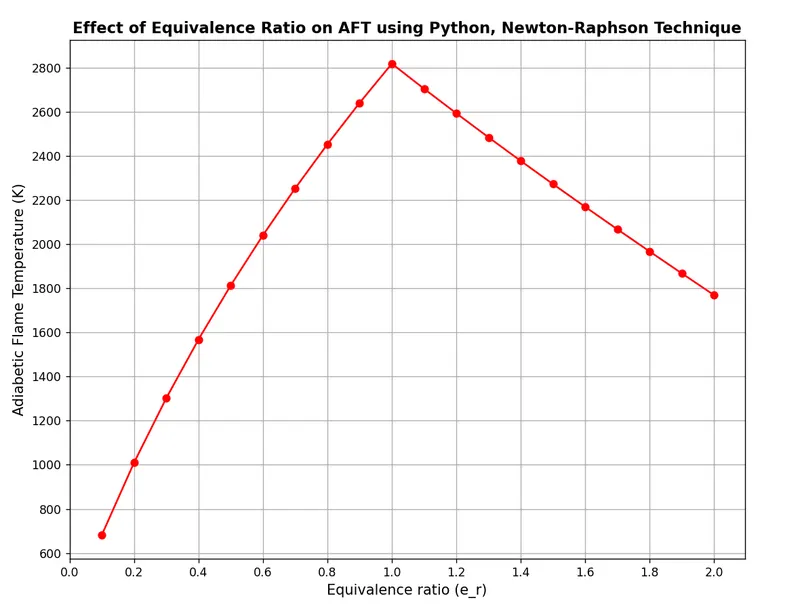
From the above figure, we can observe the range of equivalence ratios is 0.1 to 2.0 and we can observe their effect on the Adiabatic Flame Temperature. Flame temperature increases with an increase in equivalence ratio till `e_r = 1`. Beyond `e_r = 1`, flame temperature decreases with the equivalence ratio. We can see the maximum adiabatic flame temperature achieved for this combustion when the Equivalence ratio (`e_r`) is 1.0. So it can be concluded that the AFT is maximum at the stoichiometric mixture and gets low as we make the mixture lean or rich.

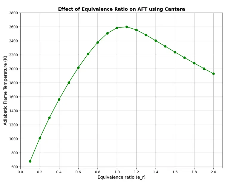
Flame temperature increases with an increase in equivalence ratio till `e_r = 1.1`. Beyond `e_r = 1.1`, flame temperature decreases with the equivalence ratio. `We can see the maximum adiabatic flame temperature achieved for this combustion when the Equivalence ratio (`e_r`) is 1.1

Comparison:

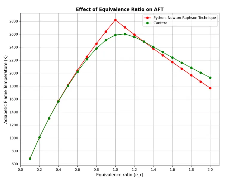
Equivalence ratio ( `phi`)	AFT using Python	AFT using Cantera
0.1	681.6845835964688	679.6185875635008
0.2	1009.552826145898	1009.4396888958659
0.3	1301.8703693601594	1300.74903429799
0.4	1567.8621974559928	1563.5555901537082
0.5	1812.8759517941469	1802.0887899096174
0.6	2040.4161376422592	2018.3725835490868
0.7	2252.9810790597203	2211.71398508243
0.8	2452.4598892859954	2377.513792657946
0.9	2640.340983400382	2506.6728691638295
1.0	2817.831019503983	2585.8782667050837
1.1	2704.1671319661473	2600.539166550205
1.2	2592.954045588545	2556.491324238801
1.3	2484.005206906715	2484.0651369968946
1.4	2377.1327939946286	2403.2562513080215
1.5	2272.1474451071	2321.02855094366
1.6	2168.858039715615	2239.5504491856113
1.7	2067.0713957627213	2159.51535304297
1.8	1966.5917891895651	2081.1419124469744
1.9	1867.2202292067605	2004.4839526412202
2.0	1768.7534362855683	1929.5327242242863

It can be observed from the above table, Maximum Adiabatic Flame Temperature obtained using Python is 2817.831019503983 K when the Equivalence ratio was 1.

It can be observed from the above table, Maximum Adiabatic Flame Temperature obtained using Cantera is 2600.539166550205 K when the Equivalence ratio was 1.1

The decrease in the adiabatic flame temperature, obtained using Cantera, can be observed as compared to Python. This is due to the process through which Cantera solves, it uses the Gibbs free energy principle. Another reason is that many species are formed in Cantera that are not considered in the Python program. Meaning, In the Python program on the product side, we consider only some species but actually in real combustion lot of intermediate reactions happen to produce many species, though their concentration can be very small, they are present in combustion products. So the process, in which Cantera solves, includes all of that into account. The reason behind less temperature is that heat produced in combustion is utilized to heat up the other gases produced during combustion.

CASE 2. Flame temperature variation with Heat loss (In constant pressure-chamber):

In this case, we are considering a constant pressure reactor with heat loss. Due to the heat loss, the reaction is no longer adiabatic and hence we will refer to the AFT as just FT (Flame Temperature). The reactor is initially set at STP conditions. We will vary the heat loss term by multiplying the "maximum heat loss" with a factor known as the Heat loss factor.

The combustion takes place in a constant pressure chamber with heat loss hence the equilibrium condition (root finding function) for the reaction is:

`H_(Products) - H_(Reactants) + Heat_(Loss) = 0`

CODE: Python code to calculate Flame temperature variation with Heat loss:

"""
Programm to find out the Flame temperature variation with heat loss (In constant pressure-chamber)
methane: CH4 + 2(O2 + 3.76N2) = CO2 + 2H2O + 7.52N2
"""

import matplotlib.pyplot as plt
import numpy as np

# Function to evaluate enthalpy
def h(T,co_effs):
	
	R = 8.314 # J/mol-K
	a1 = co_effs[0]
	a2 = co_effs[1]
	a3 = co_effs[2]
	a4 = co_effs[3]
	a5 = co_effs[4]
	a6 = co_effs[5]
	return (a1 + a2*T/2 + a3*pow(T,2)/3 + a4*pow(T,3)/4 +  a5*pow(T,4)/5 + a6/T)*R*T

# Low temperature coefficients (Reactants) at STP condition
CH4_coeffs_l = [5.14987613E+00,-1.36709788E-02,4.91800599E-05,-4.84743026E-08,1.66693956E-11,-1.02466476E+04,-4.64130376E+00]
O2_coeffs_l = [3.78245636E+00,-2.99673416E-03,9.84730201E-06,-9.68129509E-09,3.24372837E-12,-1.06394356E+03,3.65767573E+00]
N2_coeffs_l = [0.03298677E+02,0.14082404E-02,-0.03963222E-04,0.05641515E-07,-0.02444854E-10,-0.10208999E+04,0.03950372E+02]

# High-temperature coefficients (Products)
CO2_coeffs_h = [3.85746029E+00,4.41437026E-03,-2.21481404E-06,5.23490188E-10,-4.72084164E-14,-4.87591660E+04,2.27163806E+00]
H2O_coeffs_h = [3.03399249E+00,2.17691804E-03,-1.64072518E-07,-9.70419870E-11,1.68200992E-14,-3.00042971E+04,4.96677010E+00]
N2_coeffs_h = [0.02926640E+02,0.14879768E-02,-0.05684760E-05,0.10097038E-09,-0.06753351E-13,-0.09227977E+04,0.05980528E+02]

# Standard temperature condition
Tstp = 298.15 # Kelvin

# Computing the maximum possible heat loss
MHL = h(Tstp,CH4_coeffs_l) + 2*h(Tstp,O2_coeffs_l) - h(Tstp,CO2_coeffs_h) - 2*h(Tstp,H2O_coeffs_h)

# Function that represents root-finding problem
def f(T,HL_factor):

	# Calculation of enthalpy of Reactants
	h_CH4_r = h(Tstp,CH4_coeffs_l)
	h_O2_r = h(Tstp,O2_coeffs_l)
	h_N2_r = h(Tstp,N2_coeffs_l)
	H_reaactants = h_CH4_r + 2*h_O2_r + 7.52*h_N2_r

	# Calculation of enthalpy of Products
	h_CO2_p = h(T,CO2_coeffs_h)
	h_H2O_p = h(T,H2O_coeffs_h)
	h_N2_p = h(T,N2_coeffs_h)
	H_products = h_CO2_p + 2*h_H2O_p + 7.52*h_N2_p

	Heat_loss = HL_factor*MHL
	return H_products - H_reaactants + Heat_loss

# Numerical derivative of the function, used forward diffrencing technique
def fprime(T,HL_factor):
	return (f(T+1e-6, HL_factor) - f(T, HL_factor))/(1e-6)


# Using Newton-Raphson to solve iteratively
T_guess = 1500
tol = 1e-3
ct = 0
alpha = 0.9
HL_factor = np.linspace(0,1,21)
FT=[]


for i in range (0,len(HL_factor)):
		while abs(f(T_guess, HL_factor[i])) >= tol :
			T_guess = T_guess - alpha*((f(T_guess,HL_factor[i])/fprime(T_guess,HL_factor[i])))
			ct=ct+1
		FT.append(T_guess)


print(MHL)
print(FT)

# Plotting the results
plt.plot(HL_factor, FT, '-o', color='green')
plt.xlabel('Heat Loss Factor',fontsize=12)
plt.ylabel('Flame Temperature',fontsize=12)
plt.xticks(np.arange(0, 1.1, step=0.1))
plt.yticks(np.arange(200, 2400, step=200))
plt.title('Effect of Heat Loss Factor on Flame Temperature',fontsize=13,fontweight='bold')
plt.grid('on')
plt.show()

RESULT:

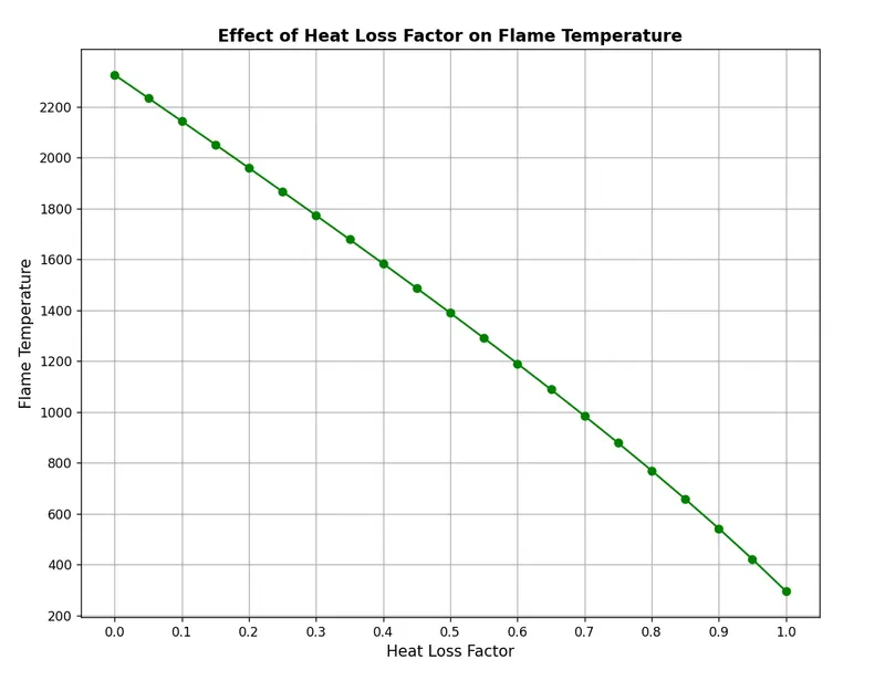
Here it can be noticed that with an increase in heat loss factor the flame temperature decreases because heat is getting lost from the system. When the heat loss factor is zero the flame temperature is 2325.59812 K and when the heat loss factor is 1 the flame temperature drops to 295.94821 K. So it is important to keep its value as low as possible.

CASE 3. Adiabatic flame temperature variation with respect to Alkane, Alkene, Alkyne:

Alkane: `C_nH_(2n+2)`

Alkene: `C_nH_(2n)`

Alkyne: `C_nH_(2n-2)`

Here we will see for Alk -ane, -ene and, -yne variants of 2 Carbon atom chains

when n=2, we will have:

Ethane: `C_2H_6`

Ethene: `C_2H_4`

Ethyne: `C_2H_2`

The stoichiometric combustion reactions for Ethane, Ethene and, Ethyne are:

Ethane:

`C_2H_6 + 3.5(O_2 + 3.76N_2) -> 2CO_2 + 3H_2O + 13.16N_2`

Ethene:

`C_2H_4 + 3(O_2 + 3.76N_2) -> 2CO_2 + 2H_2O + 11.28N_2`

Ethyne:

`C_2H_2 + 2.5(O_2 + 3.76N_2) -> 2CO_2 + H_2O + 9.4N_2`

Now we will study the Adiabatic Flame Temperature of Ethane, Ethene and, Ethyne to see how the AFT varies with the type of hydrocarbon.

The combustion takes place in a constant pressure chamber without any heat loss. Hence the equilibrium condition (root-finding function) for all the above reactions is:

`H_(Products) - H_(Reactants) = 0`

CODE: Python and Cantera code to calculate Adiabatic Flame Temperature variation with Ethane, Ethene and, Ethyne:

"""
Program to study the dependence of the Adiabatic Flame Temperature on the type of Hydrocarbon (when n=2)
General Hydrpcarbon: CxHy + [x+(y/4)](O2+3.76N2) <=> xCO2 + (y/2)H2O + 3.76[x+(y/4)]N2
Ethane: C2H6 + 3.5(O2+3.76N2) <=> 2CO2 + 3H2O + 13.16N2
Ethene: C2H4 + 3(O2+3.76N2) <=> 2CO2 + 2H2O + 11.28N2
Ethyne: C2H2 + 2.5(O2+3.76N2) <=> 2CO2 + H2O + 9.4N2
"""

import matplotlib.pyplot as plt

# Function to evaluate enthalpy
def h(T,co_effs):
	
	R = 8.314 # J/mol-K
	a1 = co_effs[0]
	a2 = co_effs[1]
	a3 = co_effs[2]
	a4 = co_effs[3]
	a5 = co_effs[4]
	a6 = co_effs[5]
	return (a1 + a2*T/2 + a3*pow(T,2)/3 + a4*pow(T,3)/4 +  a5*pow(T,4)/5 + a6/T)*R*T

# Low temperature coefficients (Reactants) at STP condition
C2H6_coeffs_l = [4.29142492E+00,-5.50154270E-03,5.99438288E-05,-7.08466285E-08,2.68685771E-11,-1.15222055E+04,2.66682316E+00]
C2H4_coeffs_l = [3.95920148E+00,-7.57052247E-03,5.70990292E-05,-6.91588753E-08,2.69884373E-11,5.08977593E+03,4.09733096E+00]
C2H2_coeffs_l = [8.08681094E-01,2.33615629E-02,-3.55171815E-05,2.80152437E-08,-8.50072974E-12,2.64289807E+04,1.39397051E+01]
O2_coeffs_l = [3.78245636E+00,-2.99673416E-03,9.84730201E-06,-9.68129509E-09,3.24372837E-12,-1.06394356E+03,3.65767573E+00]
N2_coeffs_l = [0.03298677E+02,0.14082404E-02,-0.03963222E-04,0.05641515E-07,-0.02444854E-10,-0.10208999E+04,0.03950372E+02]

# High-temperature coefficients (Products)
CO2_coeffs_h = [3.85746029E+00,4.41437026E-03,-2.21481404E-06,5.23490188E-10,-4.72084164E-14,-4.87591660E+04,2.27163806E+00]
H2O_coeffs_h = [3.03399249E+00,2.17691804E-03,-1.64072518E-07,-9.70419870E-11,1.68200992E-14,-3.00042971E+04,4.96677010E+00]
N2_coeffs_h = [0.02926640E+02,0.14879768E-02,-0.05684760E-05,0.10097038E-09,-0.06753351E-13,-0.09227977E+04,0.05980528E+02]

# Standard temperature condition
Tstp = 298.15 # K

# Function that represents root-finding problem
def f(T, ntype):

	# Calculation of enthalpy of Reactants
	h_C2H6_r = h(Tstp, C2H6_coeffs_l)
	h_C2H4_r = h(Tstp, C2H4_coeffs_l)
	h_C2H2_r = h(Tstp, C2H2_coeffs_l)
	h_O2_r = h(Tstp, O2_coeffs_l)
	h_N2_r = h(Tstp, N2_coeffs_l)

	# Calculation of enthalpy of Products
	h_CO2_p = h(T, CO2_coeffs_h)
	h_H2O_p = h(T, H2O_coeffs_h)
	h_N2_p = h(T, N2_coeffs_h)

	if ntype==1:
		H_reactants = h_C2H6_r + 3.5*(h_O2_r+3.76*h_N2_r)
		H_products = 2*h_CO2_p + 3*h_H2O_p + 13.16*h_N2_p
				

	elif ntype==2:
		H_reactants = h_C2H4_r + 3*(h_O2_r+3.76*h_N2_r)
		H_products = 2*h_CO2_p + 2*h_H2O_p + 11.28*h_N2_p
				

	elif ntype==3:
		H_reactants = h_C2H2_r + 2.5*(h_O2_r+3.76*h_N2_r)
		H_products = 2*h_CO2_p + h_H2O_p + 9.4*h_N2_p
			
	return H_products - H_reactants


# Numerical derivative of the function, used forward diffrencing technique 
def fprime(T, ntype):
		return (f(T+1e-6, ntype) - f(T, ntype))/(1e-6)

# Newton-Raphson solver
alpha = 1
tol = 1e-3
ntype = [1, 2, 3]
AFT_py = []
for i in range(0,len(ntype)):
		T_guess = 1500 
		while abs(f(T_guess, ntype[i])) >= tol:
				T_guess = T_guess - alpha*((f(T_guess,ntype[i])/fprime(T_guess,ntype[i])))
		AFT_py.append(T_guess)
		
print(AFT_py)

# Plotting the Python results
Hydrocarbon = ['Alkane (Ethane $C_2H_6$)','Alkene (Ethene $C_2H_4$)','Alkyne (Ethyne $C_2H_2$)']
plt.bar(Hydrocarbon,AFT_py,width=0.5,fc='gray',ec='black')
for i in range(0,len(ntype)):
	plt.text(i, AFT_py[i], AFT_py[i], ha='center', va='bottom',fontweight='bold')
plt.xlabel('Type of Hydrocarbon',fontsize=12)
plt.ylabel('Adiabatic Flame Temperature [K]',fontsize=12)
plt.title('AFT vs Type of Hydrocarbon (Python)',fontsize=13,fontweight='bold')
plt.show()


"""
The solution obtained by Cantera
"""
import cantera as ct

gas = ct.Solution('gri30.xml')
AFT_ct = []

for i in range (0,len(ntype)):

	# Computing the mole fractions of each reactant
	if ntype[i]==1:
		x = 2
		y = 6
		fuel = 'C2H6'
	elif ntype[i]==2:
		x = 2
		y = 4
		fuel = 'C2H4'
	elif ntype[i]==3:
		x = 2
		y = 2
		fuel = 'C2H2'

	n_Tot = 1 + (x+y/4) + 3.76*(x+y/4)
	n_fuel = 1/n_Tot
	n_O2 = (x+y/4)/n_Tot
	n_N2 = (3.76*(x+y/4))/n_Tot

	# Defining the Gas mixture
	gas.TPX = 298.15, 101325, {fuel:n_fuel, 'O2':n_O2, 'N2':n_N2}

	# Calculating the equilibrium conditions
	gas.equilibrate('HP','auto')
	AFT_ct.append(gas.T)

print(AFT_ct)

# Plotiing the Cantera results
Hydrocarbon = ['Alkane (Ethane $C_2H_6$)','Alkene (Ethene $C_2H_4$)','Alkyne (Ethyne $C_2H_2$)']
plt.bar(Hydrocarbon,AFT_ct,width=0.5,fc='gray',ec='black')
for i in range(0,len(ntype)):
	plt.text(i, AFT_ct[i], AFT_ct[i], ha='center', va='bottom',fontweight='bold')
plt.xlabel('Type of Hydrocarbon',fontsize=12)
plt.ylabel('Adiabatic Flame Temperature [K]',fontsize=12)
plt.title('AFT vs Type of Hydrocarbon (Cantera)',fontsize=13,fontweight='bold')
plt.show()

RESULT:

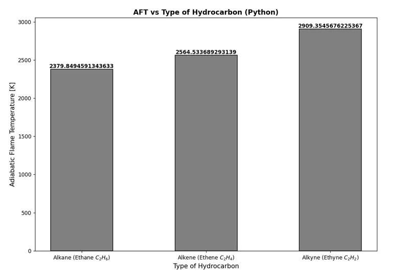
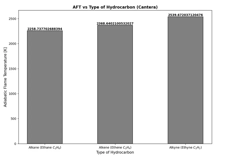
As Alkanes have only single bonds, Alkenes contain a carbon-carbon double bond and, Alkynes contain a carbon-carbon triple bond.

It can be observed from the above figures, the adiabatic flame temperature increases as the number of carbon-carbon bonds increases. Adiabatic Flame Temperature increases in "Alkane<Alkene<Alkyne" order. Alkyne (Ethyne `C_2H_2`) is found to have the highest flame temperature. This is due to the triple bonds between the carbon atoms in the fuel chemical structure. The highest flame temperature is because breaking all three bonds requires the highest amount of heat compared to the rest.

CASE 4. Adiabatic flame temperature variation with respect to the number of Carbon atom chains:

The general formula of Alkane: `C_nH_(2n+2)`

In this case, we will see the effect of the number of carbon atoms from 1 to 3 on the final temperature.

When n=1, we will have Methane: `CH_4`

When n=2, we will have Ethane: `C_2H_6`

When n=3, we will have Propane: `C_3H_8`

The stoichiometric combustion reactions for Methane, Ethane and, Propane are:

Methane:

`CH_4 + 2(O_2 + 3.76N_2) -> CO_2 + 2H_2O + 7.52N_2`

Ethane:

`C_2H_6 + 3.5(O_2 + 3.76N_2) -> 2CO_2 + 3H_2O + 13.16N_2`

Propane:

`C_3H_8 + 5(O_2 + 3.76N_2) -> 3CO_2 + 4H_2O + 18.8N_2`

Now we will study the Adiabatic Flame Temperature of Methane, Ethane and, Propane to see how the AFT varies with the number of Carbon atoms in a Hydrocarbon.

The combustion takes place in a constant pressure chamber without any heat loss. Hence the equilibrium condition (root-finding function) for all the above reactions is:

`H_(Products) - H_(Reactants) = 0`

CODE: Python and Cantera code to calculate Adiabatic Flame Temperature variation with Methane, Ethane and, Propane:

"""
Program to study the dependence of Adiabatic Flame Temperature on Number of Carbon Atoms for Alkanes
General Hydrpcarbon: CxHy + [x+(y/4)](O2+3.76N2) <=> xCO2 + (y/2)H2O + 3.76[x+(y/4)]N2
Methane: CH4 + 2(O2+3.76N2) <=> CO2 + 2H2O + 7.52N2
Ethane: C2H6 + 3.5(O2+3.76N2) <=> 2CO2 + 3H2O + 13.16N2
Propane: C3H8 + 5(O2+3.76N2) <=> 3CO2 + 4H2O + 18.8N2
"""
import matplotlib.pyplot as plt
import cantera as cantera


# Function to evaluate enthalpy 
def h(T,co_effs):
	
	R = 8.314 # J/mol-K
	a1 = co_effs[0]
	a2 = co_effs[1]
	a3 = co_effs[2]
	a4 = co_effs[3]
	a5 = co_effs[4]
	a6 = co_effs[5]
	return (a1 + a2*T/2 + a3*pow(T,2)/3 + a4*pow(T,3)/4 +  a5*pow(T,4)/5 + a6/T)*R*T

# Low temperature coefficients (Reactants) at STP condition
CH4_coeffs_l = [5.14987613E+00,-1.36709788E-02,4.91800599E-05,-4.84743026E-08,1.66693956E-11,-1.02466476E+04,-4.64130376E+00]
C2H6_coeffs_l = [4.29142492E+00,-5.50154270E-03,5.99438288E-05,-7.08466285E-08,2.68685771E-11,-1.15222055E+04,2.66682316E+00]
C3H8_coeffs_l = [0.93355381E+00,0.26424579E-01,0.61059727E-05,-0.21977499E-07,0.95149253E-11,-0.13958520E+05,0.19201691E+02]
O2_coeffs_l = [3.78245636E+00,-2.99673416E-03,9.84730201E-06,-9.68129509E-09,3.24372837E-12,-1.06394356E+03,3.65767573E+00]
N2_coeffs_l = [0.03298677E+02,0.14082404E-02,-0.03963222E-04,0.05641515E-07,-0.02444854E-10,-0.10208999E+04,0.03950372E+02]

# High-temperature coefficients (Products)
CO2_coeffs_h = [3.85746029E+00,4.41437026E-03,-2.21481404E-06,5.23490188E-10,-4.72084164E-14,-4.87591660E+04,2.27163806E+00]
H2O_coeffs_h = [3.03399249E+00,2.17691804E-03,-1.64072518E-07,-9.70419870E-11,1.68200992E-14,-3.00042971E+04,4.96677010E+00]
N2_coeffs_h = [0.02926640E+02,0.14879768E-02,-0.05684760E-05,0.10097038E-09,-0.06753351E-13,-0.09227977E+04,0.05980528E+02]

# Standard temperature condition
Tstp = 298.15 # K

# Function that represents root-finding problem
def f(T, n):
		
	# Calculation of enthalpy of Reactants
	h_CH4_r = h(Tstp, CH4_coeffs_l)
	h_C2H6_r = h(Tstp, C2H6_coeffs_l)
	h_C3H8_r = h(Tstp, C3H8_coeffs_l)
	h_O2_r = h(Tstp, O2_coeffs_l)
	h_N2_r = h(Tstp, N2_coeffs_l)

	# Calculation of enthalpy of Products
	h_CO2_p = h(T, CO2_coeffs_h)
	h_H2O_p = h(T, H2O_coeffs_h)
	h_N2_p = h(T, N2_coeffs_h)

	if n==1:
		H_reactants = h_CH4_r + 2*(h_O2_r+3.76*h_N2_r)
		H_products = h_CO2_p + 2*h_H2O_p + 7.52*h_N2_p
				

	elif n==2:
		H_reactants = h_C2H6_r + 3.5*(h_O2_r+3.76*h_N2_r)
		H_products = 2*h_CO2_p + 3*h_H2O_p + 13.16*h_N2_p
				

	elif n==3:
		H_reactants = h_C3H8_r + 5*(h_O2_r+3.76*h_N2_r)
		H_products = 3*h_CO2_p + 4*h_H2O_p + 18.8*h_N2_p
				
	return H_products - H_reactants

# Numerical derivative of the function, used forward diffrencing technique 
def fprime(T, n):
	return (f(T+1e-6, n) - f(T, n))/(1e-6)

# Newton-Raphson solver
alpha = 1
tol = 1e-3
n = [1, 2, 3]
AFT_py = []
for i in range(0,len(n)):
		T_guess = 1500 
		while abs(f(T_guess, n[i])) >= tol:
				T_guess = T_guess - alpha*((f(T_guess,n[i])/fprime(T_guess,n[i])))
		AFT_py.append(T_guess)
		
print(AFT_py)

# Plotting the Python results
Alkane = ['Methane $CH_4$(n=1)','Ethane $C_2H_6$(n=2)','Propane $C_3H_8$(n=3)']
plt.bar(Alkane,AFT_py,width=0.5,fc='gray',ec='black')
for i in range(0,len(n)):
	plt.text(i, AFT_py[i], AFT_py[i], ha='center', va='bottom',fontweight='bold')
plt.ylabel('Adiabatic Flame Temperature [K]',fontsize=12)
plt.title('AFT vs Number of Carbon atoms - Alkanes (Python)',fontsize=13,fontweight='bold')
plt.show()


"""
The solution obtained by Cantera
"""
import cantera as ct

gas = ct.Solution('gri30.xml')
AFT_ct = []

for i in range (0,len(n)):
	
	# Computing the mole fractions of each reactant
	if n[i]==1:
		x = 1
		y = 4
		fuel = 'CH4'
	elif n[i]==2:
		x = 2
		y = 6
		fuel = 'C2H6'
	elif n[i]==3:
		x = 3
		y = 8
		fuel = 'C3H8'

	n_Tot = 1 + (x+y/4) + 3.76*(x+y/4)
	n_fuel = 1/n_Tot
	n_O2 = (x+y/4)/n_Tot
	n_N2 = (3.76*(x+y/4))/n_Tot

	# Defining the Gas mixture
	gas.TPX = 298.15, 101325, {fuel:n_fuel, 'O2':n_O2, 'N2':n_N2}

	# Calculating the equilibrium conditions
	gas.equilibrate('HP','auto')
	AFT_ct.append(gas.T)

print(AFT_ct)

# Plotiing the Cantera results
Alkane = ['Methane $CH_4$(n=1)','Ethane $C_2H_6$(n=2)','Propane $C_3H_8$(n=3)']
plt.bar(Alkane,AFT_ct,width=0.5,fc='gray',ec='black')
for i in range(0,len(n)):
	plt.text(i, AFT_ct[i], AFT_ct[i], ha='center', va='bottom',fontweight='bold')
plt.ylabel('Adiabatic Flame Temperature [K]',fontsize=12)
plt.title('AFT vs Number of Carbon atoms - Alkanes (Cantera)',fontsize=13,fontweight='bold')
plt.show()

RESULT:

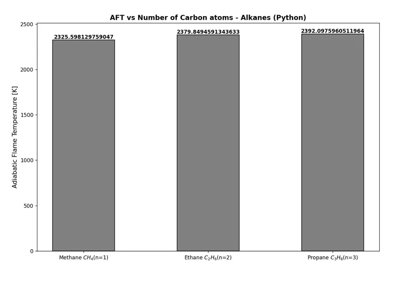
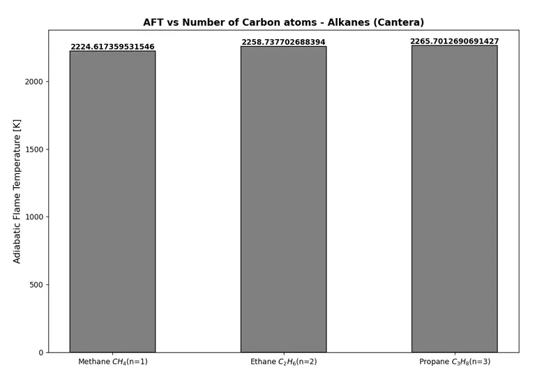
It can be observed from the above figures, the adiabatic flame temperature increases as the number of carbon atoms increases. Adiabatic Flame Temperature increases in "Methane<Ethane<Propane" order. Propane `C_3H_8`(n=3) is found to have the highest flame temperature. This is due to the higher number of carbon and hydrogen atoms.

It can also be noticed that the adiabatic flame temperature for methane is lower than that one calculated in the first case. In the first case, the adiabatic flame temperature was calculated, for Methane in the constant volume chamber. Here in the fourth case as the adiabatic flame temperature was calculated in the constant pressure chamber. Here we found that the adiabatic flame temperature for Methane, in the constant volume chamber, is higher than the adiabatic flame temperature for methane in the constant pressure chamber. This is because the constant volume adiabatic flame temperature considers that no energy is employed in changing the volume of the system. Hence, we have a greater value of AFT for a constant volume chamber.

CONCLUSIONS: We can have some conclusions from all the above four cases:

The adiabatic flame temperature of the stoichiometric mixture is higher than that of the lean and rich mixture.
Heat loss during combustion results in a drop in adiabatic flame temperature.
Alkyne has the highest flame temperature as compared to Alkene and Alkane due to more carbon bonds.
Adiabatic flame temperature increases as the number of carbon atoms increases.
Lesser value of all Cantera results, in the cases, makes us think about the influence of many species that formed during the combustion reaction.

Week 3 - Adiabatic Flame Temperature calculation

Ship work like this
in your own course.

Talk to a career counsellor

Ship work like thisin your own course.

Talk to a career counsellor

Ship work like this
in your own course.