Week 3 - Adiabatic Flame Temperature calculation
Adiabetic Flame Temperature:-
When a combustion reaction takes place energy is liberated to the combustion products. If no heat is lost in this process, the temperature of the combustion products is known as the "Adiabatic Flame Temperature." This is the maximum temperature that can be reached for given reactants.
Types of Air-Fuel Mixture:-
Stoichiometric Combustion:-
The air-fuel ratio for complete combustion is called the stoichiometric air-fuel ratio.
Lean Combustion:-
If the amount of air is more than fuel for complete combustion. this is called lean combustion.
Rich Combustion:-
If the amount of fuel is more than air for complete combustion. this is called rich combustion.
Equivalence Ratio:-
The equivalence ratio is the ratio between the oxygen content in the oxidant supply and that required for complete stoichiometric combustion. It is likely the most significant operating parameter for all thermal processes since it strongly influences the gas composition and its heating value.
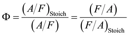
General equation for Hydrocarbon Combustion:-
CxHy + [x + (y/4)]*[O2 +3.76N2] = xCO2 + (y/2)*H2O + 3.76[x+ (y/4)]*N2
Coding Method:-
Newton Raphson method is used. The enthalpy of products and reactants is calculated using NASA polynomial.
H = ((a1 + a2*T/2 + a3*pow(T,2)/3 + a4*pow(T,3)/4 + a5*pow(T,4)/5 + a6/T)*R*T)
Coefficients for the above polynomial are obtained from Berkely(UCLA) website.
1. Adiabatic flame temperature variation with Equivalence ratio (In constant volume-chamber) :
"""
Program for Calculating Adiabetic Flame temperature ot methane with different Equivalnce ratio
# Stoichometric Mixture
CH4 + 2( O2 + 3.76N2) = Co2 + 2H2o + 7.5N2

#Lean Mixture
CH4 + (2/phi)*( O2 + 3.76N2) = Co2 + 2H2o + (2/phi-2)*o2 + (7.52/phi)N2

#Rich Mixture
CH4 + (2/phi)*( O2 + 3.76N2) = (4/phi-3)*Co2 + 2H2o + (4-4/phi)*o2 + (7.52/phi)N2

"""

import matplotlib.pyplot as plt
import math
import numpy as np

def h(T,co_effs):

	"""
	Function to evaluate enthalpy
	"""
	R = 8.314 #J/mol-k
	a1 = co_effs[0]
	a2 = co_effs[1]
	a3 = co_effs[2]
	a4 = co_effs[3]
	a5 = co_effs[4]
	a6 = co_effs[5]

	return (a1 + a2*T/2 + a3*pow(T,2)/3 + a4*pow(T,3)/4 + a5*pow(T,4)/5 + a6/T)*R*T

#low temperature coefficients
ch4_coeffs_l = [5.14987613E+00,-1.36709788E-02, 4.91800599E-05,-4.84743026E-08, 1.66693956E-11,-1.02466476E+04,-4.64130376E+00 ]

o2_coeffs_l = [3.78245636E+00,-2.99673416E-03, 9.84730201E-06,-9.68129509E-09, 3.24372837E-12,-1.06394356E+03, 3.65767573E+00 ]

n2_coeffs_l = [0.03298677E+02, 0.14082404E-02,-0.03963222E-04,0.05641515E-07,-0.02444854E-10,-0.10208999E+04, 0.03950372E+02 ]

#high temperature coefficients
o2_coeffs_h = [3.28253784E+00, 1.48308754E-03,-7.57966669E-07, 2.09470555E-10,-2.16717794E-14,-1.08845772E+03, 5.45323129E+00]

n2_coeffs_h = [0.02926640E+02, 0.1487976E-02,-0.05684760E-05, 0.10097038E-09,-0.06753351E-13,-0.09227977E+04, 0.05980528E+02]

co2_coeffs_h = [3.85746029E+00, 4.41437026E-03,-2.21481404E-06, 5.23490188E-10,-4.72084164E-14,-4.87591660E+04, 2.27163806E+00 ]

h2o_coeffs_h = [3.03399249E+00, 2.17691804E-03,-1.64072518E-07,-9.70419870E-11, 1.68200992E-14,-3.00042971E+04, 4.96677010E+00 ]

co_coeffs_h = [2.71518561E+00, 2.06252743E-03,-9.98825771E-07, 2.30053008E-10,-2.03647716E-14,-1.41518724E+04, 7.81868772E+00]


def f(T):
	"""
	Function that represents root finding problem
	"""

	h_co2_p = h(T,co2_coeffs_h)
	h_n2_p = h(T,n2_coeffs_h)
	h_h2o_p = h(T,h2o_coeffs_h)
	h_o2_p = h(T,o2_coeffs_h)
	h_co_p = h(T,co_coeffs_h)

	R = 8.314

	# Lean Mixture
	if phi < 1:
			H_products = h_co2_p + 2*h_h2o_p + (7.52/phi)*h_n2_p + ((2/phi)-2)*h_o2_p
			n_products = 1 + (7.52/phi) + 2 + ((2/phi)-2)

	if phi == 1:
			H_products = h_co2_p + 2*h_h2o_p + 7.52*h_n2_p
			n_products = 1 + 7.52 + 2

	if phi > 1:
			H_products = ((4/phi)-3)*h_co2_p + 2*h_h2o_p + (7.52/phi)*h_n2_p + (4-(4/phi))*h_co_p
			n_products = ((4/phi)-3) + 2 + (7.52/phi) + (4-(4/phi))

	Tstd = 298.15
	h_ch4_r = h(Tstd,ch4_coeffs_l)
	h_o2_r = h(Tstd,o2_coeffs_l)
	h_n2_r = h(Tstd,n2_coeffs_l)

	H_reactants = (h_ch4_r + (2/phi)*(h_o2_r) + (3.76*h_n2_r))
	n_reactants = 1 + (2/phi) + (3.76*(2/phi))

	return (H_products - n_products*R*T) - (H_reactants - n_reactants*R*Tstd)

def fprime(T):
	return (f(T+1e-6) - f(T))/1e-6


# Newton Raphson Method
T_guess = 1500
alpha = 0.2
tol = 1e-6
X = np.arange(0.1,2,0.05)
T_ad = []


for phi in X:
		while(abs(f(T_guess)) > tol):
				T_guess = T_guess - alpha*((f(T_guess)/fprime(T_guess)))

		T_ad.append(T_guess)


plt.plot(X,T_ad,color='red',label="Using Newton Raphson Method")
plt.grid('on')


#Program using Cantera

import cantera as ct
T_adc =[]
for phi in np.arange(0.1,2,0.05):
	gas = ct.Solution('gri30.xml')
	gas.TPX = 298.15,101325,{'CH4':1,'O2':2/phi,'N2':7.52/phi}
	gas.equilibrate('Uv','auto')
	T_adc.append(gas.T)

plt.plot(X,T_adc,color='blue',label='Using Cantera')
plt.xlabel('Equivalence Ratio')
plt.ylabel('Adiabetic Flame Temperature in K')
plt.title('Equivalence ratio vs Adiabetic Flame Temperature')
plt.legend()
plt.show()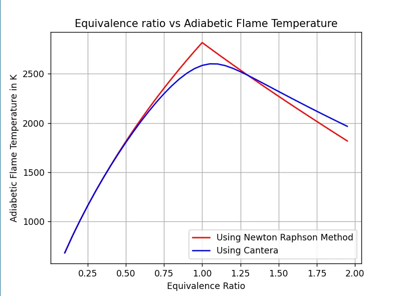
Figure(1)
From the above plot, it is clear stoichiometric combustion reaches the highest temperature than others, by the complete combustion of fuel and producing more energy. Cantera gives AFT temperatures than the newton raphson method because Cantera evaluates all products of the combustion, so more energy is used to produce this product.
2. Flame temperature variation with Heat loss:-
"""
Adiabetic Flame Temperature

CH4 + 2( O2 + 3.76N2) = Co2 + 2H2o + 7.5N2
"""

import matplotlib.pyplot as plt
import math
import numpy as np

def h(T,co_effs):

	"""
	Function to evaluate enthalpy
	"""
	R = 8.314 #J/mol-k
	a1 = co_effs[0]
	a2 = co_effs[1]
	a3 = co_effs[2]
	a4 = co_effs[3]
	a5 = co_effs[4]
	a6 = co_effs[5]

	return (a1 + a2*T/2 + a3*pow(T,2)/3 + a4*pow(T,3)/4 + a5*pow(T,4)/5 + a6/T)*R*T

#low temperature coefficients
ch4_coeffs_l = [5.14987613E+00,-1.36709788E-02, 4.91800599E-05,-4.84743026E-08, 1.66693956E-11,-1.02466476E+04,-4.64130376E+00]

o2_coeffs_l = [3.78245636E+00,-2.99673416E-03, 9.84730201E-06,-9.68129509E-09, 3.24372837E-12,-1.06394356E+03, 3.65767573E+00]

n2_coeffs_l = [0.03298677E+02, 0.14082404E-02,-0.03963222E-04,0.05641515E-07,-0.02444854E-10,-0.10208999E+04, 0.03950372E+02]

#high temperature coefficients
o2_coeffs_h = [3.28253784E+00, 1.48308754E-03,-7.57966669E-07, 2.09470555E-10,-2.16717794E-14,-1.08845772E+03, 5.45323129E+00]

n2_coeffs_h = [0.02926640E+02, 0.1487976E-02,-0.05684760E-05, 0.10097038E-09,-0.06753351E-13,-0.09227977E+04, 0.05980528E+02]

co2_coeffs_h = [3.85746029E+00, 4.41437026E-03,-2.21481404E-06, 5.23490188E-10,-4.72084164E-14,-4.87591660E+04, 2.27163806E+00]

h2o_coeffs_h = [3.03399249E+00, 2.17691804E-03,-1.64072518E-07,-9.70419870E-11, 1.68200992E-14,-3.00042971E+04, 4.96677010E+00]

co_coeffs_h = [2.71518561E+00, 2.06252743E-03,-9.98825771E-07, 2.30053008E-10,-2.03647716E-14,-1.41518724E+04, 7.81868772E+00]

Tstd = 298.15 #K

#Calculating the maximum possible heat loss

#LHV = Heat Loss Factor
LHV = h(Tstd,ch4_coeffs_l) + 2*h(Tstd,o2_coeffs_l) - h(Tstd,co2_coeffs_h) - 2*h(Tstd,h2o_coeffs_h)

def f(T,Heat_Loss):
	"""
	Function that represents root finding problem
	"""
	h_co2_p = h(T,co2_coeffs_h)
	h_n2_p = h(T,n2_coeffs_h)
	h_h2o_p = h(T,h2o_coeffs_h)

	H_products = h_co2_p + 2*h_h2o_p + 7.52*h_n2_p

	h_ch4_r = h(Tstd,ch4_coeffs_l)
	h_o2_r = h(Tstd,o2_coeffs_l)
	h_n2_r = h(Tstd,n2_coeffs_l)

	H_reactants = h_ch4_r + 2*(h_o2_r + 3.76*h_n2_r)

	return (H_products - H_reactants + (Heat_Loss*LHV))

def fprime(T,Heat_Loss):
	return (f(T+1e-6,Heat_Loss) - f(T,Heat_Loss))/1e-6


# Newton Raphson Method
T_guess = 1500
alpha = 0.2
tol = 1e-6
Heat_Loss = np.linspace(0,1,10)
temp = []


for i in range(0,len(Heat_Loss)):
		while(abs(f(T_guess,Heat_Loss[i])) > tol):
				T_guess = T_guess - alpha*((f(T_guess,Heat_Loss[i])/fprime(T_guess,Heat_Loss[i])))
		temp.append(T_guess)

#plotting
plt.plot(Heat_Loss,temp,color='black')
plt.plot(Heat_Loss[3],temp[3],'*',color='red',label='Heat Loss')
plt.grid('on')
plt.legend()
plt.xlabel('Heat Loss Factor')
plt.ylabel('Adiabetic Flame Temperature')
plt.title('Heat Loss Factor vs Adiabetic Flame Temperature')
plt.show()
Figure(1)
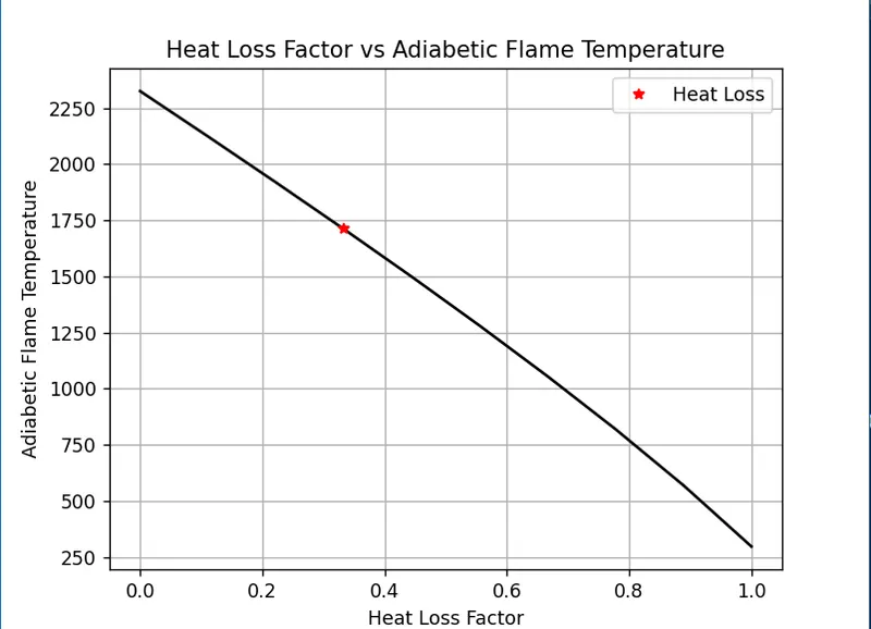
From the above plot is clear that, as heat loss increases, AFT decreases due to energy loss.
3. Adiabatic flame temperature variation with respect to Alkane, Alkene, Alkyne :
"""
Adiabetic Flame Temperature variation for Alkane, Alkene, and Alkyne

# Alkane - Ethane
C2H6 + 3.5*(O2 + 3.76N2) = 2CO2 + 3H2O + 13.16N2

#Alkene - Ethene
C2H4 + 3*(O2 + 3.76N2)= 2CO2 + 2H2O + 11.28N2

#Alkyne - Ethyne
C2H2 + 2.5*(O2 + 3.76N2)= 2CO2 + H2O + 9.4N2

#General Hydrocarbon reaction:
CxHy + [x + (y/4)]*[O2 +3.76N2] = xCO2 + (y/2)*H2O + 3.76[x+ (y/4)]*N2

"""
import matplotlib.pyplot as plt

def h(T,co_effs):

	"""
	Function to evaluate enthalpy
	"""
	R = 8.314 #J/mol-k
	a1 = co_effs[0]
	a2 = co_effs[1]
	a3 = co_effs[2]
	a4 = co_effs[3]
	a5 = co_effs[4]
	a6 = co_effs[5]

	return (a1 + a2*T/2 + a3*pow(T,2)/3 + a4*pow(T,3)/4 + a5*pow(T,4)/5 + a6/T)*R*T

#low temperature coefficients

c2h6_coeffs_l = [4.29142492E+00,-5.50154270E-03, 5.99438288E-05,-7.08466285E-08, 2.68685771E-11,-1.15222055E+04, 2.66682316E+00]

c2h4_coeffs_l = [3.95920148E+00,-7.57052247E-03, 5.70990292E-05,-6.91588753E-08, 2.69884373E-11, 5.08977593E+03, 4.09733096E+00]

c2h2_coeffs_l = [8.08681094E-01, 2.33615629E-02,-3.55171815E-05,2.80152437E-08,-8.50072974E-12, 2.64289807E+04, 1.39397051E+01]

o2_coeffs_l = [3.78245636E+00,-2.99673416E-03, 9.84730201E-06,-9.68129509E-09, 3.24372837E-12,-1.06394356E+03, 3.65767573E+00]

n2_coeffs_l = [0.03298677E+02, 0.14082404E-02,-0.03963222E-04,0.05641515E-07,-0.02444854E-10,-0.10208999E+04, 0.03950372E+02]

#high temperature coefficients
co2_coeffs_h = [3.85746029E+00, 4.41437026E-03,-2.21481404E-06, 5.23490188E-10,-4.72084164E-14,-4.87591660E+04, 2.27163806E+00]

h2o_coeffs_h = [3.03399249E+00, 2.17691804E-03,-1.64072518E-07,-9.70419870E-11, 1.68200992E-14,-3.00042971E+04, 4.96677010E+00]

n2_coeffs_h = [0.02926640E+02, 0.1487976E-02,-0.05684760E-05, 0.10097038E-09,-0.06753351E-13,-0.09227977E+04, 0.05980528E+02]

#Stabders Temperature
Tstd = 298.15 #K

def f(T,ntype):
	"""
	Function that represents root finding problem
	"""

	h_co2_p = h(T,co2_coeffs_h)
	h_n2_p = h(T,n2_coeffs_h)
	h_h2o_p = h(T,h2o_coeffs_h)

	h_c2h6_r = h(Tstd,c2h6_coeffs_l)
	h_c2h4_r = h(Tstd,c2h4_coeffs_l)
	h_c2h2_r = h(Tstd,c2h2_coeffs_l)
	h_o2_r = h(Tstd,o2_coeffs_l)
	h_n2_r = h(Tstd,n2_coeffs_l)

	if ntype == 1:
		x = 2
		y = 6
		h_fuel = h_c2h6_r

	elif ntype == 2:
		x = 2
		y = 4
		h_fuel = h_c2h4_r

	elif ntype == 3:
		x = 2
		y = 2
		h_fuel = h_c2h2_r

	H_products = x*h_co2_p + (y/2)*h_h2o_p + 3.76*(x + y/4)*h_n2_p

	H_reactants = h_fuel +  (x + y/4)*h_o2_r + 3.76*(x + y/4)*h_n2_r

	return (H_products - H_reactants)

def fprime(T,ntype):
	return (f(T+1e-6,ntype) - f(T,ntype))/1e-6

# Newton Raphson Method
T_guess = 1500
alpha = 0.2
tol = 1e-6
ntype = [1,2,3]
temp = []


for i in range(0,len(ntype)):
		while(abs(f(T_guess,ntype[i])) > tol):
				T_guess = T_guess - alpha*((f(T_guess,ntype[i])/fprime(T_guess,ntype[i])))
		temp.append(T_guess)

#plotting
plt.figure(1)
plt.bar(['Ethane($C_2H_6$)','Ethene($C_2H_4$)','Ethyne($C_2H_2$)'],temp)
plt.ylabel('Adiabetic Flame Temperature')
plt.title('Adiabetic Flame Temperature for Ethane, Ethene and Ethyne')
plt.show()


"""
Adiabetic Flame Temperature variation for Alkane, Alkene, and Alkyne using Cantera
"""
import cantera as ct

gas = ct.Solution('gri30.xml')
t = []

for i in range(0,len(ntype)):
	if ntype[i] == 1:
		x = 2
		y = 6
		fuel = 'C2H6'
	elif ntype[i] == 2:
		x = 2
		y = 4
		fuel ='C2H4'

	elif ntype[i] == 3:
		x = 2
		y = 2
		fuel = 'C2H2'

	n_tot = 1 +(x +y/4) + 3.76*(x +y/4)
	n_fuel = 1/n_tot
	n_o2 = (x +y/4)/n_tot
	n_n2 = 3.76*(x +y/4)/n_tot


	gas.TPX = 298.15,101325,{fuel:n_fuel,'O2':n_o2,'N2':n_n2}
	gas.equilibrate('HP','auto')
	t.append(gas.T)

plt.figure(2)
plt.bar(['Ethane($C_2H_6$)','Ethene($C_2H_4$)','Ethyne($C_2H_2$)'],t)
plt.ylabel('Adiabetic Flame Temperature')
plt.title('Adiabetic Flame Temperature for Ethane, Ethene and Ethyne using Cantera')
plt.show() 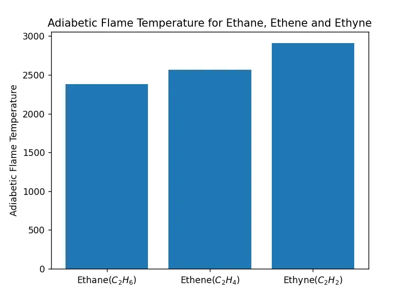
Figure(1)
Figure(2)
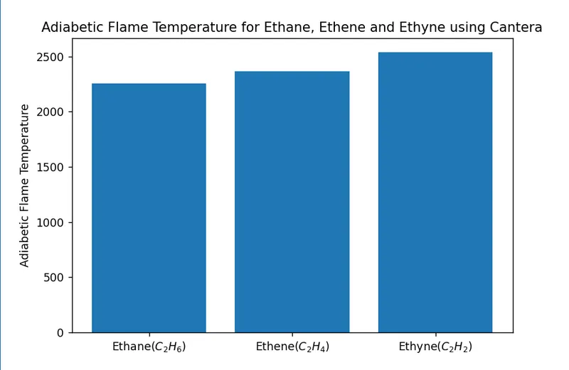
From the above graphs, it is observed that the highest temperature is achieved by ethyne followed by ethene, and the lowest temperature is achieved by ethane.
4. Adiabatic flame temperature variation with respect to number of Carbon atom chains :
"""
Adiabatic flame temperature variation with respect to number of Carbon atom chains

# Alkane - Methane
CH4 + 2( O2 + 3.76N2) = Co2 + 2H2o + 7.5N2

#Alkane - Ethene
C2H6 + 3.5*(O2 + 3.76N2)= 2CO2 + 3H2O + 13.16N2

#Alkane - Propane
C3H8 + 5*(O2 + 3.76N2)= 3CO2 + 4H2O + 18.8N2

"""
import matplotlib.pyplot as plt

def h(T,co_effs):

	"""
	Function to evaluate enthalpy
	"""
	R = 8.314 #J/mol-k
	a1 = co_effs[0]
	a2 = co_effs[1]
	a3 = co_effs[2]
	a4 = co_effs[3]
	a5 = co_effs[4]
	a6 = co_effs[5]

	return (a1 + a2*T/2 + a3*pow(T,2)/3 + a4*pow(T,3)/4 + a5*pow(T,4)/5 + a6/T)*R*T

#low temperature coefficients
ch4_coeffs_l = [5.14987613E+00,-1.36709788E-02, 4.91800599E-05,-4.84743026E-08, 1.66693956E-11,-1.02466476E+04,-4.64130376E+00]

c2h6_coeffs_l = [4.29142492E+00,-5.50154270E-03, 5.99438288E-05,-7.08466285E-08, 2.68685771E-11,-1.15222055E+04, 2.66682316E+00]

c3h8_coeffs_l = [0.93355381E+00, 0.26424579E-01, 0.61059727E-05,-0.21977499E-07, 0.95149253E-11,-0.13958520E+05, 0.19201691E+02]

o2_coeffs_l = [3.78245636E+00,-2.99673416E-03, 9.84730201E-06,-9.68129509E-09, 3.24372837E-12,-1.06394356E+03, 3.65767573E+00]

n2_coeffs_l = [0.03298677E+02, 0.14082404E-02,-0.03963222E-04,0.05641515E-07,-0.02444854E-10,-0.10208999E+04, 0.03950372E+02]


#high temperature coefficients
co2_coeffs_h = [3.85746029E+00, 4.41437026E-03,-2.21481404E-06, 5.23490188E-10,-4.72084164E-14,-4.87591660E+04, 2.27163806E+00]

h2o_coeffs_h = [3.03399249E+00, 2.17691804E-03,-1.64072518E-07,-9.70419870E-11, 1.68200992E-14,-3.00042971E+04, 4.96677010E+00]

n2_coeffs_h = [0.02926640E+02, 0.1487976E-02,-0.05684760E-05, 0.10097038E-09,-0.06753351E-13,-0.09227977E+04, 0.05980528E+02]

#Stabders Temperature
Tstd = 298.15 #K

def f(T,ntype):
	"""
	Function that represents root finding problem
	"""

	h_co2_p = h(T,co2_coeffs_h)
	h_n2_p = h(T,n2_coeffs_h)
	h_h2o_p = h(T,h2o_coeffs_h)

	h_ch4_r = h(Tstd,ch4_coeffs_l)
	h_c2h6_r = h(Tstd,c2h6_coeffs_l)
	h_c3h8_r = h(Tstd,c3h8_coeffs_l)
	h_o2_r = h(Tstd,o2_coeffs_l)
	h_n2_r = h(Tstd,n2_coeffs_l)

	if ntype == 1:
		x = 1
		y = 4
		h_fuel = h_ch4_r

	elif ntype == 2:
		x = 2
		y = 6
		h_fuel = h_c2h6_r

	elif ntype == 3:
		x = 3
		y = 8
		h_fuel = h_c3h8_r


	H_products = x*h_co2_p + (y/2)*h_h2o_p + 3.76*(x + y/4)*h_n2_p

	H_reactants = h_fuel +  (x + y/4)*h_o2_r + 3.76*(x + y/4)*h_n2_r

	return (H_products - H_reactants)

def fprime(T,ntype):
	return (f(T+1e-6,ntype) - f(T,ntype))/1e-6

# Newton Raphson Method
T_guess = 1500
alpha = 0.2
tol = 1e-6
ntype = [1,2,3]
temp = []


for i in range(0,len(ntype)):
		while(abs(f(T_guess,ntype[i])) > tol):
				T_guess = T_guess - alpha*((f(T_guess,ntype[i])/fprime(T_guess,ntype[i])))
		temp.append(T_guess)

#plotting
plt.figure(1)
plt.bar(['Methane($CH_4$)','Ethane($C_2H_6$)','Propane($C_3H_8$)'],temp)
plt.ylabel('Adiabetic Flame Temperature')
plt.title('Adiabetic Flame Temperature for Methane, Ethane and Propane')
plt.show()


"""
Adiabetic Flame Temperature variation for different Alkanes using Cantera
"""
import cantera as ct

gas = ct.Solution('gri30.xml')
t = []

for i in range(0,len(ntype)):
	if ntype[i] == 1:
		x = 1
		y = 4
		fuel = 'CH4'
	elif ntype[i] == 2:
		x = 2
		y = 6
		fuel ='C2H6'

	elif ntype[i] == 3:
		x = 3
		y = 8
		fuel = 'C3H8'

	n_tot = 1 +(x +y/4) + 3.76*(x +y/4)
	n_fuel = 1/n_tot
	n_o2 = (x +y/4)/n_tot
	n_n2 = 3.76*(x +y/4)/n_tot


	gas.TPX = 298.15,101325,{fuel:n_fuel,'O2':n_o2,'N2':n_n2}
	gas.equilibrate('HP','auto')
	t.append(gas.T)

#plotting
plt.figure(2)
plt.bar(['Methane($CH_4$)','Ethane($C_2H_6$)','Propane($C_3H_8$)'],t)
plt.ylabel('Adiabetic Flame Temperature')
plt.title('Adiabetic Flame Temperature for Methane, Ethane and Propane using Cantera')
plt.show()
Output plots:-
Figure(1)
Figure(2)
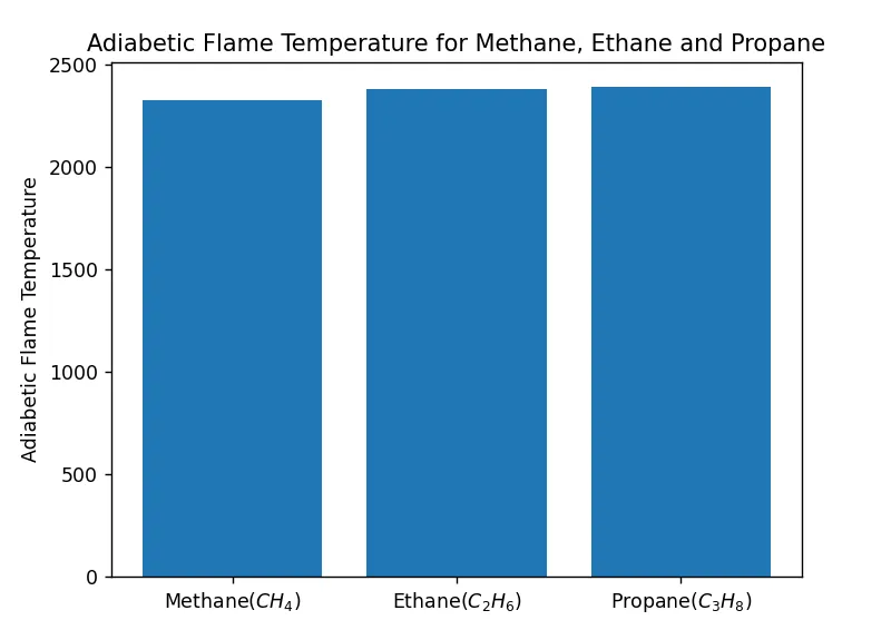
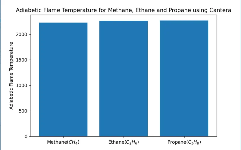
From the above graphs, it is observed that the highest temperature is achieved by propane and the lowest temperature is achieved by methane.