Week 3 - Adiabatic Flame Temperature calculation
Aim --> To calculate AFT (Adiabatic flame temperature) and its variation using python and Cantera.
Objectives -->
- Adiabatic flame temperature variation with Equivalence ratio (In constant volume-chamber).
- Adiabatic flame temperature variation with Heat loss (In constant pressure chamber with heat loss).
- Adiabatic flame temperature variation with respect to Alkane, Alkene, Alkyne.
- Adiabatic flame temperature variation with respect to a number of Carbon atom chains.
Theory
--> According to the 1st law of thermodynamics, Adiabatic Flame Temperature is defined for constant pressure and constant volume combustion process. If a given uniform mixture with an initial temperature and composition is made to approach chemical equilibrium through an adiabatic, isobaric process at pressure p, then the final temperature is the adiabatic flame temperature, Tad. All the heat from the combustion is used to increase the sensible enthalpies of the products, this happens if there is no heat loss to surroundings. Also, we are saying that final products are at equilibrium. This quantity is of importance in the study of combustion because it directly affects the reactivity of the various chemical processes including those involving pollutant formation.
- Constant Pressure Adiabatic Flame Temperature (AFT) is calculated at isobaric conditions (volume is allowed to change). Enthalpy of reactants is equal to enthalpy of products. The final temperature attained by the products is the AFT at constant pressure.
 Q(p) = 0 for adiabatic condition (no heat loss)
- Constant Volume Adiabatic Flame Temperature (AFT) is calculated at isochoric conditions (pressure changes). Internal Energy (U) of reactants is equal to the Internal Energy of products. The final temperature attained by the products is the AFT at constant volume.
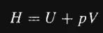 and from Ideal gas relations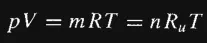

Equivalence Ratio
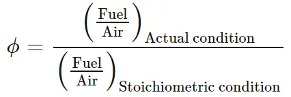
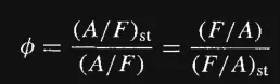
--> It is defined as the ratio of actual fuel-oxidant ratio [F/O] to the ratio [F/O] (fuel-oxidant) for a stoichiometric process. A stoichiometric reaction is the most economic reaction in which the oxidizer is just the amount required to completely burn the quantity of fuel in the system.
CASE I
- Adiabatic flame temperature variation with Equivalence ratio (In constant volume-chamber).
General Stoichiometric Reaction
CxHy + (x + y/4)(O2 + 3.76*N2) ----> xCO2 + (y/2)H2O + ((x + y/4)*3.76)N2
Python code
#[PART 1]
""""
Program to calculate the AFT variation with Equivalence ratio (phi).
for phi = 1 (stoichiometric)     CH4 + 2 [ O2 + 3.76 N2 ] ----->  CO2 + 2 H2O + 7.52 N2

for phi < 1 (LEAN)     CH4 + 2/(PHI) [ O2 + 3.76 N2 ] ----->  CO2 + 2 H2O + 7.52/(PHI) N2 + [ 2/(PHI) - 2 ] O2

for phi > 1 (RICH)     CH4 + 2/(PHI) [ O2 + 3.76 N2 ] ----->  [ 4/(PHI) - 3 ] CO2 + 2 H2O + 7.52/(PHI) N2
                                                                                     +  [ 4 - 4/(PHI) ] CO
"""
import matplotlib.pyplot as plt
import math
import numpy

T1 = 298.15   # Kelvin Initial Temperature at standard conditions
R = 8.314  # KJ / [mol-K]
# Calculating the enthalpy using NASA Polynomials.

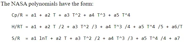
def h(T, coe_effs):
    """
        Function to calculate the enthalpy
        inputs --> Temperature and coefficient of polynomials
    """
    R = 8.314  # KJ / [mol-K]
    a1 = coe_effs[0]
    a2 = coe_effs[1]
    a3 = coe_effs[2]
    a4 = coe_effs[3]
    a5 = coe_effs[4]
    a6 = coe_effs[5]

    return (a1 + a2*T/2 + a3*pow(T, 2)/3 + a4*pow(T, 3)/4 + a5*pow(T, 4)/5 + a6/T )*R*T

phi = numpy.linspace(0.1,2.0,200)
T = numpy.zeros(200)

ch4_coffs_l = [5.14987613E+00, -1.36709788E-02, 4.91800599E-05, -4.84743026E-08, 1.66693956E-11, -1.02466476E+04, -4.64130376E+00]
o2_coffs_l = [3.78245636E+00, -2.99673416E-03, 9.84730201E-06, -9.68129509E-09, 3.24372837E-12, -1.06394356E+03, 3.65767573E+00]
o2_coffs_h = [3.28253784E+00, 1.48308754E-03, -7.57966669E-07, 2.09470555E-10, -2.16717794E-14, -1.08845772E+03, 5.45323129E+00]
n2_coffs_l = [0.03298677E+02, 0.14082404E-02, -0.03963222E-04, 0.05641515E-07, -0.02444854E-10, -0.10208999E+04, 0.03950372E+02]
n2_coffs_h = [0.02926640E+02, 0.14879768E-02, -0.05684760E-05, 0.10097038E-09, -0.06753351E-13, -0.09227977E+04, 0.05980528E+02]
co2_coffs_h = [3.85746029E+00, 4.41437026E-03, -2.21481404E-06, 5.23490188E-10, -4.72084164E-14, -4.87591660E+04, 2.27163806E+00]
h2o_coffs_h = [3.03399249E+00, 2.17691804E-03, -1.64072518E-07, -9.70419870E-11, 1.68200992E-14, -3.00042971E+04, 4.96677010E+00]
co_coffs_h = [2.71518561E+00, 2.06252743E-03, -9.98825771E-07, 2.30053008E-10, -2.03647716E-14, -1.41518724E+04, 7.81868772E+00]

for i in range(len(phi)):
    if phi[i] < 1:
        """
        for phi<1[LEAN]  /////  CH4 + 2/(PHI) [ O2 + 3.76 N2 ] ----->  CO2 + 2 H2O + 7.52/(PHI) N2 + [ 2/(PHI) - 2 ] O2
        """
        def f(T, i):
            h_ch4_r = h(T1, ch4_coffs_l)
            h_o2_r = h(T1, o2_coffs_l)
            h_n2_r = h(T1, n2_coffs_l)
            h_r =  h_ch4_r  +  2/(phi[i])*h_o2_r  +  2/(phi[i])*3.76*h_n2_r
            print(h_r)

            h_co2_p = h(T, co2_coffs_h)
            h_h20_p = h(T, h2o_coffs_h)
            h_n2_p = h(T, n2_coffs_h)
            h_o2_p = h(T, o2_coffs_h)
            h_p = h_co2_p + 2*h_h20_p + 7.52/(phi[i])*h_n2_p + (2/(phi[i]) - 2)*h_o2_p
            print(h_p)

            pv_term = R*(T1*(1 + 2/phi[i] + 2*3.76/phi[i]) - T*(3 + 7.52/phi[i] + (2/phi[i] - 2)))
            print(pv_term)

            return h_r - h_p - pv_term
        def fprime(T, i):
            return (f(T+1e-6, i) - f(T, i))/1e-6
        T_guess = 1600
        tol = 1e-3
        ct = 0
        alpha = 0.2
        while (abs(f(T_guess, i)) > tol):
            T_guess = T_guess - alpha*(f(T_guess, i)/fprime(T_guess, i))
            ct = ct + 1
        print(ct)
        print(T_guess)
        T[i] = T_guess
    elif phi[i] == 1:
        """
        for phi=1[STOICHIOMETRIC]  ///// CH4 + 2 [ O2 + 3.76 N2 ] ----->  CO2 + 2 H2O + 7.52 N2
        """
        def f(T, i):
            h_ch4_r = h(T1, ch4_coffs_l)
            h_o2_r = h(T1, o2_coffs_l)
            h_n2_r = h(T1, n2_coffs_l)
            h_r = h_ch4_r + 2*h_o2_r + 2*3.76*h_n2_r
            print(h_r)
            h_co2_p = h(T, co2_coffs_h)
            h_h20_p = h(T, h2o_coffs_h)
            h_n2_p = h(T, n2_coffs_h)
            h_p = h_co2_p + 2*h_h20_p + 7.52*h_n2_p
            print(h_p)
            pv_term = R*(T1*(1 + 2 + 2*3.76) - T*(3 + 7.52 ))
            print(pv_term)
            return h_r - h_p - pv_term
        def fprime(T, i):
            return (f(T+1e-6, i) - f(T, i))/1e-6
        T_guess = 1600
        tol = 1e-3
        ct = 0
        alpha = 0.2
        while (abs(f(T_guess, i)) > tol):
            T_guess = T_guess - alpha * (f(T_guess, i) / fprime(T_guess, i))
            ct = ct + 1
        print(ct)
        print(T_guess)
        T[i] = T_guess
    else:
        """
        for phi>1(RICH)   CH4 + 2/(PHI)[O2+3.76N2] ---> [4/(PHI)-3]CO2 + 2H2O + 7.52/(PHI)N2 + [4-4/(PHI)]CO
        """
        def f(T, i):
            h_ch4_r = h(T1, ch4_coffs_l)
            h_o2_r = h(T1, o2_coffs_l)
            h_n2_r = h(T1, n2_coffs_l)
            h_r = h_ch4_r + 2/(phi[i])*h_o2_r + 2/phi[i]*3.76*h_n2_r
            print(h_r)

            h_co2_p = h(T, co2_coffs_h)
            h_h20_p = h(T, h2o_coffs_h)
            h_n2_p = h(T, n2_coffs_h)
            h_co_p = h(T, co_coffs_h)
            h_p = (4/phi[i] - 3)*h_co2_p + 2*h_h20_p + 7.52/phi[i]*h_n2_p + (4 - 4/phi[i])*h_co_p
            print(h_p)

            pv_term = R*(T1*(1 + 2/phi[i] + 2*3.76/phi[i]) - T*(3 + 7.52/phi[i]))
            print(pv_term)

            return h_r - h_p - pv_term
        def fprime(T, i):
            return (f(T+1e-6, i) - f(T, i))/1e-6
        T_guess = 1600
        tol = 1e-3
        ct = 0
        alpha = 0.2
        while (abs(f(T_guess, i)) > tol):
            T_guess = T_guess - alpha*(f(T_guess, i)/fprime(T_guess, i))
            ct = ct + 1
        print(ct)
        print(T_guess)
        T[i] = T_guess
print(phi,T)
plt.plot(phi,T)
plt.xlabel('Equivalence ratio "phi"')
plt.ylabel('Temperature')
plt.grid('on')

#[PART 2]
# Program to calculate the AFT variation with Equivalence ratio (phi) using Cantera.
import cantera as ct
gas = ct.Solution('gri30.xml')
n = 200
Phi = numpy.linspace(0.1,2.0,n)
t = numpy.zeros(n)
for i in range(n):
    gas.set_equivalence_ratio(Phi[i], 'CH4', 'O2:1.0, N2:3.76')
    gas.TP = 298.15,101325
    gas.equilibrate('UV','auto')
    t[i] = gas.T
print(Phi,t)
plt.plot(Phi,t)
plt.legend(('Python','Cantera'))
plt.show()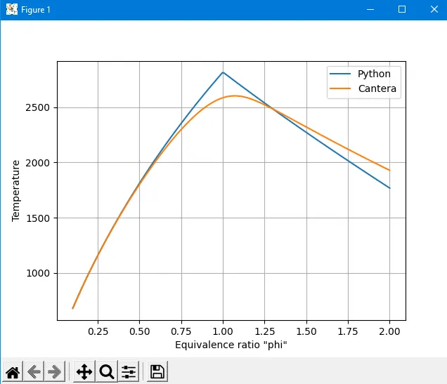
--> Using python code gives us the highest AFT at phi = 1. For Cantera, as it is a chemical kinetics library it will have more species on the products side the AFT will be less and it occurs between 1-1.25.
CASE II
- Adiabatic flame temperature variation with Heat loss (In constant pressure chamber with heat loss).
--> We assume an Equivalence ratio equal of 1. We are aiming to capture variation in AFT with heat loss at the isobaric condition. Here stoichiometric combustion of Methane is given by (CH4) the following equation.

Calculation of Maximum Heat loss (Assume 100% efficiency for Max. Heat loss)
Fuel efficiency --> 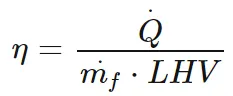
The lower heating value (LHV) (net calorific value (NCV) or lower calorific value (LCV)) is another measure of available thermal energy produced by combustion of fuel, measured as a unit of energy per unit mass or volume of a substance. The total amount of heat liberated during the combustion of a unit of fuel, the HHV or HCV, includes the latent heat stored in the vapourised water.
mf = 16.04 g/mol
LHV = 50 MJ/Kg
Python code
"""
Adiabatic flame temperature variation with Heat loss (In constant pressure chamber).
Consider a constant pressure reactor with heat loss. The reactor is initially set at STP conditions.

The heat loss should be input in your program and must be a fraction of the "maximum possible heat
loss". You will control heat loss using a variable called H_loss. For example, H_loss = 0.5 would mean a heat loss that is equal to 50% of the maximum possible heat loss.

The fuel type can be a general hydrocarbon of the form CxHy. Phi and lambda = 1.0.
Find the AFT of CH4 with H_loss = 0.35
"""

import numpy
import matplotlib.pyplot as plt
import math

T1 = 298.15   # Kelvin Initial Temperature at standard conditions
R = 8.314  # KJ / [mol-K]
phi = 1 # Equivalence Ratio Stoichiometric Combustion
# for phi=1[STOICHIOMETRIC]  ///// CH4 + 2 [ O2 + 3.76 N2 ] ----->  CO2 + 2 H2O + 7.52 N2
Q_max = 80200 # Maximum Heat loss

def h(T, coe_effs):
    """
        Function to calculate the enthalpy
        inputs --> Temperature and coefficient of polynomials
    """
    R = 8.314  # KJ / [mol-K]
    a1 = coe_effs[0]
    a2 = coe_effs[1]
    a3 = coe_effs[2]
    a4 = coe_effs[3]
    a5 = coe_effs[4]
    a6 = coe_effs[5]

    return (a1 + a2*T/2 + a3*pow(T, 2)/3 + a4*pow(T, 3)/4 + a5*pow(T, 4)/5 + a6/T )*R*T
N=200
H_loss = numpy.linspace(0.1,1.0,N)
T = numpy.zeros(N)

ch4_coffs_l = [5.14987613E+00, -1.36709788E-02, 4.91800599E-05, -4.84743026E-08, 1.66693956E-11, -1.02466476E+04, -4.64130376E+00]
o2_coffs_l = [3.78245636E+00, -2.99673416E-03, 9.84730201E-06, -9.68129509E-09, 3.24372837E-12, -1.06394356E+03, 3.65767573E+00]
o2_coffs_h = [3.28253784E+00, 1.48308754E-03, -7.57966669E-07, 2.09470555E-10, -2.16717794E-14, -1.08845772E+03, 5.45323129E+00]
n2_coffs_l = [0.03298677E+02, 0.14082404E-02, -0.03963222E-04, 0.05641515E-07, -0.02444854E-10, -0.10208999E+04, 0.03950372E+02]
n2_coffs_h = [0.02926640E+02, 0.14879768E-02, -0.05684760E-05, 0.10097038E-09, -0.06753351E-13, -0.09227977E+04, 0.05980528E+02]
co2_coffs_h = [3.85746029E+00, 4.41437026E-03, -2.21481404E-06, 5.23490188E-10, -4.72084164E-14, -4.87591660E+04, 2.27163806E+00]
h2o_coffs_h = [3.03399249E+00, 2.17691804E-03, -1.64072518E-07, -9.70419870E-11, 1.68200992E-14, -3.00042971E+04, 4.96677010E+00]
co_coffs_h = [2.71518561E+00, 2.06252743E-03, -9.98825771E-07, 2.30053008E-10, -2.03647716E-14, -1.41518724E+04, 7.81868772E+00]

for i in range(len(H_loss)):
	def f(T, i):
		h_ch4_r = h(T1, ch4_coffs_l)
		h_o2_r = h(T1, o2_coffs_l)
		h_n2_r = h(T1, n2_coffs_l)
		h_r = h_ch4_r + 2*h_o2_r + 2*3.76*h_n2_r
		h_co2_p = h(T, co2_coffs_h)
		h_h20_p = h(T, h2o_coffs_h)
		h_n2_p = h(T, n2_coffs_h)
		h_p = h_co2_p + 2*h_h20_p + 7.52*h_n2_p
		return h_p - h_r + Q_max*H_loss[i]
	def fprime(T, i):
		return (f(T+1e-6, i) - f(T, i))/1e-6
	T_guess = 1800
	tol = 1e-3
	ct = 0
	alpha = 0.9
	while (abs(f(T_guess, i)) > tol):
		T_guess = T_guess - alpha * (f(T_guess, i) / fprime(T_guess, i)) # Newton-Raphson Method
		ct = ct + 1
		print(T_guess)
	T[i]=T_guess
print(H_loss,T)
plt.plot(H_loss,T)
plt.xlabel('Heat loss fraction of Q_max')
plt.ylabel('Temperature')
plt.grid('on')
plt.show()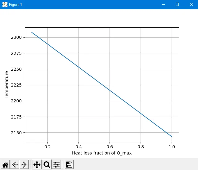
--> AFT variation is linear with a heat loss coefficient. An increase in heat loss coefficient will lead to a decrease in AFT.
CASE III
- Adiabatic flame temperature variation with respect to Alkane, Alkene, Alkyne.
Python code
"""
Adiabatic flame temperature variation with respect to Alkane, Alkene, Alkyne :

Test it only for Alk-ane, -ene and -yne variants of 2 Carbon atom
chain and plot a trend. The provided therm.dat might not contain data for other alkanes, alkynes, and alkenes (in that case use Cantera).
Assume no heat loss.
"""
import numpy
import matplotlib.pyplot as plt
import math


# Python code
T1 = 298.15   # Kelvin Initial Temperature at standard conditions
R = 8.314  # KJ / [mol-K]
phi = 1 # Equivalence Ratio Stoichiometric Combustion

def h(T, coe_effs):
    """
        Function to calculate the enthalpy
        inputs --> Temperature and coefficient of polynomials
    """
    R = 8.314  # KJ / [mol-K]
    a1 = coe_effs[0]
    a2 = coe_effs[1]
    a3 = coe_effs[2]
    a4 = coe_effs[3]
    a5 = coe_effs[4]
    a6 = coe_effs[5]

    return (a1 + a2*T/2 + a3*pow(T, 2)/3 + a4*pow(T, 3)/4 + a5*pow(T, 4)/5 + a6/T )*R*T
T = [0, 0, 0]

c2h6_coeffs_l = [4.29142492E+00, -5.50154270E-03, 5.99438288E-05, -7.08466285E-08, 2.68685771E-11, -1.15222055E+04, 2.66682316E+00]
c2h4_coeffs_l = [3.95920148E+00, -7.57052247E-03, 5.70990292E-05, -6.91588753E-08, 2.69884373E-11, 5.08977593E+03, 4.09733096E+00]
c2h2_coeffs_l = [8.08681094E-01, 2.33615629E-02, -3.55171815E-05, 2.80152437E-08, -8.50072974E-12, 2.64289807E+04, 1.39397051E+01]
o2_coffs_l = [3.78245636E+00, -2.99673416E-03, 9.84730201E-06, -9.68129509E-09, 3.24372837E-12, -1.06394356E+03, 3.65767573E+00]
n2_coffs_l = [0.03298677E+02, 0.14082404E-02, -0.03963222E-04, 0.05641515E-07, -0.02444854E-10, -0.10208999E+04, 0.03950372E+02]
n2_coffs_h = [0.02926640E+02, 0.14879768E-02, -0.05684760E-05, 0.10097038E-09, -0.06753351E-13, -0.09227977E+04, 0.05980528E+02]
co2_coffs_h = [3.85746029E+00, 4.41437026E-03, -2.21481404E-06, 5.23490188E-10, -4.72084164E-14, -4.87591660E+04, 2.27163806E+00]
h2o_coffs_h = [3.03399249E+00, 2.17691804E-03, -1.64072518E-07, -9.70419870E-11, 1.68200992E-14, -3.00042971E+04, 4.96677010E+00]

for i in range(len(T)):
    if i == 1: # ALkane ----- C2H6 + 3.5(O2 + 3.76N2) <-> 2CO2 + 3H20 + 13.16N2
        def f(T, i):
            h_c2h6_r = h(T1, c2h6_coeffs_l)
            h_o2_r = h(T1, o2_coffs_l)
            h_n2_r = h(T1, n2_coffs_l)
            h_r = h_c2h6_r + 3.5*h_o2_r + 3.5*3.76*h_n2_r
            h_co2_p = h(T, co2_coffs_h)
            h_h20_p = h(T, h2o_coffs_h)
            h_n2_p = h(T, n2_coffs_h)
            h_p = 2*h_co2_p + 3*h_h20_p + 13.16*h_n2_p
            return h_p - h_r
        def fprime(T, i):
            return (f(T+1e-6, i) - f(T, i))/1e-6
        T_guess = 1800
        tol = 1e-3
        ct = 0
        alpha = 0.9
        while (abs(f(T_guess, i)) > tol):
            T_guess = T_guess - alpha * (f(T_guess, i) / fprime(T_guess, i)) # Newton-Raphson Method
            ct = ct + 1
            print(T_guess)
        T[i-1]=T_guess
    elif i==2: # ALkene ------  C2H4 + 3(O2 + 3.76N2) <-> 2CO2 + 2H20 + 11.28N2
        def f(T, i):
            h_c2h4_r = h(T1, c2h4_coeffs_l)
            h_o2_r = h(T1, o2_coffs_l)
            h_n2_r = h(T1, n2_coffs_l)
            h_r = h_c2h4_r + 3*h_o2_r + 3*3.76*h_n2_r
            h_co2_p = h(T, co2_coffs_h)
            h_h20_p = h(T, h2o_coffs_h)
            h_n2_p = h(T, n2_coffs_h)
            h_p = 2*h_co2_p + 2*h_h20_p + 11.28*h_n2_p
            return h_p - h_r
        def fprime(T, i):
            return (f(T+1e-6, i) - f(T, i))/1e-6
        T_guess = 1600
        tol = 1e-3
        ct = 0
        alpha = 0.9
        while (abs(f(T_guess, i)) > tol):
            T_guess = T_guess - alpha * (f(T_guess, i) / fprime(T_guess, i)) # Newton-Raphson Method
            ct = ct + 1
            print(T_guess)
        T[i-1]=T_guess
    else:  # ALkyne ------- C2H2 + 2.5(O2 + 3.76N2) <-> 2CO2 + 1H20 + 9.4N2
        def f(T, i):
            h_c2h2_r = h(T1, c2h2_coeffs_l)
            h_o2_r = h(T1, o2_coffs_l)
            h_n2_r = h(T1, n2_coffs_l)
            h_r = h_c2h2_r + 2.5*h_o2_r + 2.5*3.76*h_n2_r
            h_co2_p = h(T, co2_coffs_h)
            h_h20_p = h(T, h2o_coffs_h)
            h_n2_p = h(T, n2_coffs_h)
            h_p = 2*h_co2_p + h_h20_p + 9.4*h_n2_p
            return h_p - h_r
        def fprime(T, i):
            return (f(T+1e-6, i) - f(T, i))/1e-6
        T_guess = 1600
        tol = 1e-3
        ct = 0
        alpha = 0.9
        while (abs(f(T_guess, i)) > tol):
            T_guess = T_guess - alpha * (f(T_guess, i) / fprime(T_guess, i)) # Newton-Raphson Method
            ct = ct + 1
            print(T_guess)
        T[i-1]=T_guess
plt.bar(['Alkane','Alkene','Alkyne'],T,color='red')
plt.title('Variation of AFT using Python')
plt.show()


#### Cantera code
import cantera as ct
T_cantera = [1, 2, 3]
# C2H6 + 3.5(O2 + 3.76N2) <-> 2CO2 + 3H20 + 13.16N2
gas1 = ct.Solution('gri30.xml')
gas1.TPX = 298.15, 101325, {'C2H6':1, 'O2':3.5, 'N2':13.16}
gas1.equilibrate('HP','auto')
T_cantera[0] = gas1.T
print(T_cantera[0])

# C2H4 + 3(O2 + 3.76N2) <-> 2CO2 + 2H20 + 11.28N2
gas2 = ct.Solution('gri30.xml')
gas2.TPX = 298.15, 101325, {'C2H4':1, 'O2':3, 'N2':11.28}
gas2.equilibrate('HP','auto')
T_cantera[1] = gas2.T
print(T_cantera[1])

# C2H2 + 2.5(O2 + 3.76N2) <-> 2CO2 + 1H20 + 9.4N2
gas3 = ct.Solution('gri30.xml')
gas3.TPX = 298.15, 101325, {'C2H2':1, 'O2':2.5, 'N2':9.4}
gas3.equilibrate('HP','auto')
T_cantera[2] = gas3.T
print(T_cantera[2])

plt.bar(['Alkane','Alkene','Alkyne'],T_cantera,color='red')
plt.title('Variation of AFT using Cantera')
plt.show()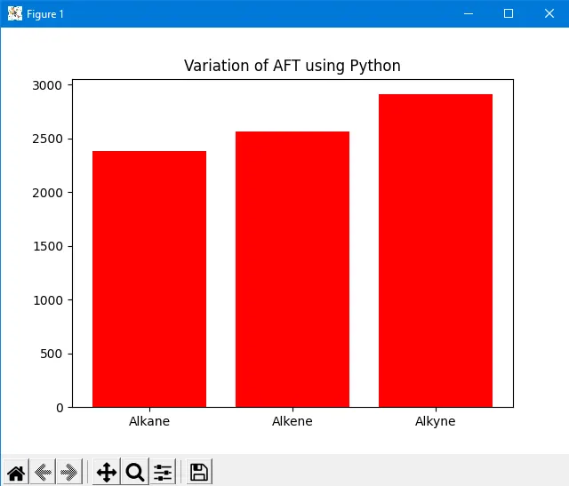
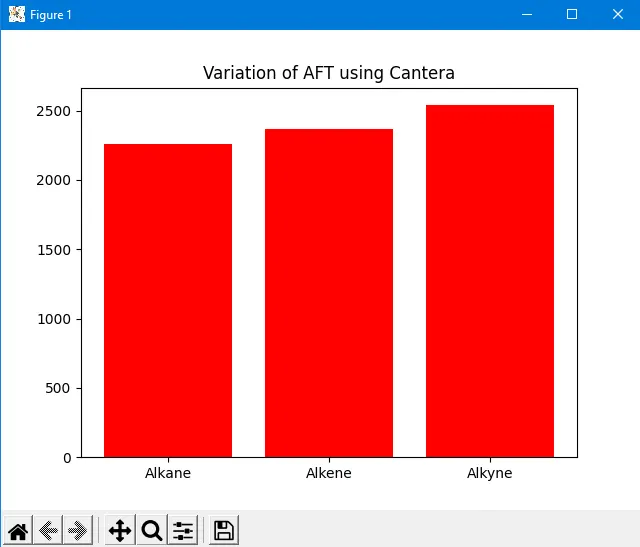
--> Lowering the number of hydrogen atoms causes less H2O production increasing AFT.
CASE IV
- Adiabatic flame temperature variation with respect to a number of Carbon atom chains.
Python code
import matplotlib.pyplot as plt
import math
import cantera as ct

# Variation of Number of Carbon Atoms

T_alkane = [1, 2, 3]

# CH4 + 2(O2 + 3.76N2) <-> 2CO2 + 3H20 + 13.16N2
gas3 = ct.Solution('gri30.xml')
gas3.TPX = 298.15, 101325, {'CH4':1, 'O2':2, 'N2':7.52}
gas3.equilibrate('HP','auto')
T_alkane[0] = gas3.T
print(T_alkane[0])

# C2H6 + 3.5(O2 + 3.76N2) <-> 2CO2 + 3H20 + 13.16N2
gas1 = ct.Solution('gri30.xml')
gas1.TPX = 298.15, 101325, {'C2H6':1, 'O2':3.5, 'N2':13.16}
gas1.equilibrate('HP','auto')
T_alkane[1] = gas1.T
print(T_alkane[1])

# C3H8 + 5(O2 + 3.76N2) <-> 2CO2 + 3H20 + 13.16N2
gas2 = ct.Solution('gri30.xml')
gas2.TPX = 298.15, 101325, {'C3H8':1, 'O2':5, 'N2':18.8}
gas2.equilibrate('HP','auto')
T_alkane[2] = gas2.T
print(T_alkane[2])

plt.bar(['CH4','C2H6','C3H8'],T_alkane,color='blue')
plt.title('Variation of AFT using Cantera')
plt.show()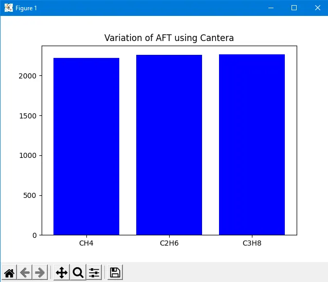
--> As the Number of Carbon atoms increases, more heat is generated. Hense C3H8 gives the highest AFT.
--> Thus we have performed a study on Adiabatic flame temperature, its variation w.r.t. equivalence ratio, heat loss with isochoric and isobaric conditions resp. We also studied the effect of alkane, alkene, alkyne, lower hydrogen atoms and variation of AFT with No. of Carbon Atoms.