Week 3 - Adiabatic Flame Temperature calculation
Adiabatic Flame Temperature calculation
Aim:
To find Adiabatic Flame Temperature of the following cases:
- Adiabatic flame temperature variation with Equivalence ratio (In constant volume chamber).
- Adiabatic flame temperature variation with Heat loss (In constant pressure chamber).
- Adiabatic flame temperature variation with respect to Alkane, Alkene, Alkyne.
- Adiabatic flame temperature variation with respect to a number of Carbon atom chains.
Theory:
Newton Raphson method:
The Newton-Raphson method (also known as Newton's method) is a way to quickly find a good approximation for the root of a real-valued function `f(x) = 0`. It uses the idea that a continuous and differentiable function can be approximated by a straight line tangent to it.
Working
Suppose you need to find the root of a continuous, differentiable function `f(x)`, and you know the root you are looking for is near the point `x = x_0`. Then Newton's method tells us that a better approximation for the root is
`x_1 = x_0 - \frac{f(x_0)}{f'(x_0)}`
This process may be repeated as many times as necessary to get the desired accuracy. In general, for any xx-value x_nxn, the next value is given by
`x_{n+1} = x_n - \frac{f(x_n)}{f'(x_n)}`.
the term "near" is used loosely because it does not need a precise definition in this context. However,`x_0` should be closer to the root you need than to any other root (if the function has multiple roots).
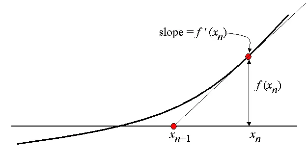
We draw a tangent line to the graph of `f(x)` at the point `x = x_n`. This line has slope `f′(x_n)` and goes through the point `(x_n, f(x_n))`. Therefore it has the equation `y = f'(x_n)(x - x_n) + f(x_n)`. Now, we find the root of this tangent line by setting `y = 0` and `x=x_{n+1}` for our new approximation. Solving this equation gives us our new approximation, which is
`x_{n+1} = x_n - \frac{f(x_n)}{f'(x_n)}`
Adiabatic Flame Temperature:
The temperature developed by the combustion of a fuel and oxidizer mixture in conditions where there are no heat losses.
The adiabatic flame temperature is one that occurs when the combustion chamber is well insulated with no heat losses (adiabatic conditions). The peak adiabatic flame temperature occurs at around Φ = 1 in an ideally insulated combustion chamber.
We define two adiabatic flame temperatures: one for constant pressure and one for constant volume combustion.
constant pressure combustion:
If the combustion takes place in a constant pressure adiabatic chamber then that combustion is called constant pressure combustion. which would be appropriate in dealing with a gas-turbine combustor, or a furnace.
To find Adiabatic Flame temperature for this process we have to equate the absolute enthalpy of reactance at the initial state and the absolute enthalpy of products at the final state.
`H_("reactant")(T_i,P)=H_("product")(T_(ad),P)`
or, equivalently, on a per-mass-of-mixture basis,
`h_("reactant")(T_i,P)=h_("product")(T_(ad),P)`
Constant volume combustion :
If the combustion takes place in a constant volume adiabatic chamber then that combustion is called constant volume combustion. which we might require in an ideal Otto-cycle analysis,
To find Adiabatic Flame temperature for this process we have to equate the Internal energy of reactance at the initial state and Internal energy products at the final state.
`U_("reactant")(T_("initial"),P_("initial"))=U_("product")(T_(ad),P_f)`
`U = H-PV`
`H("reactant")-H("product")-V(P_("init")-P_f)=0`
`P*V= N*R_U*T`
`H_("react")-H_("prod")-R_U*(N_("rect")*T_("init")-N_("prod")*T_("ad"))=0`
Stoichiometry
The stoichiometric quantity of oxidizer is just that amount needed to completely burn a quantity of fuel. If more than a stoichiometric quantity of oxidizer is supplied, the mixture is said to be lean, while supplying less than the stoichiometric oxidizer results in a rich mixture. The stoichiometric oxidizer/ fuel ratio (mass) is determined by writing simple atom balances, assuming that the fuel reacts to form an ideal set of products. For a hydrocarbon fuel given by `C_xH_y` , the stoichiometric relation can be expressed as
`CxHy + (x+y/4)*(O2+3.76*N2) -> x*Co2 + (y/2)*H2O + (x+y/4)*N2`
where
`a=x+y /4`
The stoichiometric air–fuel ratio can be found as
`(A/ F)_("stoic")= [m_(air)/m_(fuel)]_("stoic")`
Equivalance ratio `Phi`:
The equivalence ratio is commonly used to indicate quantitatively whether a fuel–oxidizer mixture is rich, lean, or stoichiometric. The equivalence ratio is defined as
`Phi = (A/F)_("stoic")/(A/F)_("fuel")=(F/A)_("fuel")/(F/A)_("stoic")`
From this definition, we see that
For fuel-rich mixtures, Φ > 1
For fuel-lean mixtures, Φ < 1.
For a stoichiometric mixture, Φ = 1.
In many combustion applications, the equivalence ratio is the single most important factor in determining a system’s performance
Python modules required:
Math: module that has to be imported to do mathematical tasks. The math module has a set of methods and constants.
Numpy: NumPy is a Python library used for working with arrays. It also has functions for working in the domain of linear algebra, Fourier transform, and matrices.
Matplotlib.pyplot: Matplotlib is an amazing visualization library in Python for 2D plots of arrays. Matplotlib is a multi-platform data visualization library built on NumPy arrays and designed to work with the broader SciPy stack.
Cantera: Cantera automates the chemical kinetic, thermodynamic, and transport calculations so that the users can efficiently incorporate detailed chemical thermo-kinetics and transport models into their calculations.
1) Adiabatic flame temperature variation with Equivalence ratio (In constant volume chamber).
Assume that methane is contained in a constant volume chamber. Write a program in Python to plot the effect of the equivalence ratio on the final adiabatic flame temperature. Compare the results with Cantera.
In this assignment, we have to find the AFT of methane CH4 for various equivalence ratios ranges from 0-2.
rich mixtures, Φ > 1
lean mixtures, Φ < 1.
stoichiometric mixture, Φ = 1.
The general form of stoichiometric equation is:
`CxHy + (x+y/4)*(O2+3.76*N2) -> x*Co2 + (y/2)*H2O + (x+y/4)*N2`
we considered methane `Cxhy=CH4` as fuel so `x= 1;y=4;a = x+y/4 = 1+4/4=2`
for lean mixtures, Φ < 1 & rich mixtures, Φ > 1
`Phi = a_("stoic")/a_("fuel") rArr a_("fuel") =a_("stoic")/Phi rArr a_("fuel") =2/Phi`
`Phi`= equivalence ratio = `e_r`
lean mixture
after equating the coefficents on both sides combustion equation for lean mixture the equation become
`CH4 + (2/e_r)*(O2+3.76*N2) -> CO2 + 2H2O + ((2/e_r)-2)O2 + (7.52/e_r)*N2`
Rich mixture
after equating the coefficents on both sides combustion equation for rich mixture the equation become
`CH4 + (2/e_r)*(O2+3.76*N2) -> ((4/e_r)-3)CO2 + 2H2O + (4-(4/e_r))CO + (7.52/e_r)*N2`
Procedure:
- import math, Numpy, Matplotlib.pyplot & Cantera libraries as modules.
- Writing a function to calculate the enthalpy of Reactance and Products using NASA Polynomial by taking temperature and Species coefficients as inputs.`H/(R*T)=a1+a2*(T/2)+a3*(T^2/3)+a4*(T^3/4)+a5*(T^4/5)+(a6)/T`
- Define the lower and higher temperature Coefficents of Reactance and Product species according to the side of involvement.
- Writing a function that calculates `H_("react")-H_("prod")-R_U*(N_("rect")*T_("init")-N_("prod")*T_("ad"))` by taking temperature and equalance ratio as inputs.
- Writing a function to calculate the 2nd order numerical derivative of the above function using the Foward differencing approach.
- Setting a for loop to calculate AFT for various Equalance ratios.
- In the for loop set a while loop to perform the Newton Raphson root finding method to calculate AFT for each Equalance ratio.
- use Cantera to find AFT for Equalance ratios.
- compare the results produced by the Newton-Raphson method and by Cantera.
- plot the results.
# Adiabatic flame temperature variation with Equivalence ratio
# (In constant volume-chamber) :
# in this program we are going to calculate the AFT of Methane at different equalance ratios

# CH4 + 2(O2+3.76N2) = CO2 + 2H2O + 7.52N2                  stoichiometric combustion
# CH4+2/er(O2+3.76N2) => CO2+2H2O+(2/er-2)O2+7.52/er*N2     Lean combustion
# CH4+2/er(O2+3.76N2) => (4/er-3)CO2+2H2O+(4-4/er)CO+7.52/er*N2  Rich combustion

import math
import matplotlib.pyplot as plt
import numpy as np
import cantera as ct

def h(T,co_eff):

	R  = 8.314 #j/mol-K
	a1 = co_eff[0]
	a2 = co_eff[1]
	a3 = co_eff[2]
	a4 = co_eff[3]
	a5 = co_eff[4]
	a6 = co_eff[5]
	return R*T*(a1 + a2*T/2 + a3*pow(T,2)/3 + a4*pow(T,3)/4 + a5*pow(T,4)/5 + a6/T)

# low temperrture coefficients
CH4_coeff_l = [5.14987613E+00, -1.36709788E-02, 4.91800599E-05, -4.84743026E-08, 1.66693956E-11, -1.02466476E+04]
O2_coeff_l  = [3.78245636E+00, -2.99673416E-03, 9.84730201E-06, -9.68129509E-09, 3.24372837E-12, -1.06394356E+03]
N2_coeff_l  = [0.03298677E+02, 0.14082404E-02, -0.03963222E-04, 0.05641515E-07, -0.02444854E-10, -0.10208999E+04]
# High temperature coefficients
CO2_coeff_h = [3.85746029E+00, 4.41437026E-03, -2.21481404E-06, 5.23490188E-10, -4.72084164E-14, -4.87591660E+04]
H20_coeff_h = [3.03399249E+00, 2.17691804E-03, -1.64072518E-07, -9.70419870E-11, 1.68200992E-14, -3.00042971E+04]
N2_coeff_h  = [0.02926640E+02, 0.14879768E-02, -0.05684760E-05, 0.10097038E-09, -0.06753351E-13, -0.09227977E+04]
O2_coeff_h  = [3.28253784E+00, 1.48308754E-03, -7.57966669E-07, 2.09470555E-10, -2.16717794E-14, -1.08845772E+03]
CO_coeff_h  = [2.71518561E+00, 2.06252743E-03, -9.98825771E-07, 2.30053008E-10, -2.03647716E-14, -1.41518724E+04]

# for  constant volume adiabatic flame temperatures
# U_reac(T_init - P_init) = U_prod(T_ad - P_f)     => U = H - pv
# H_products - H_reactance  - (pv_products - pv_reactance) = 0

def G(T,e_r):
	# Roots finding problem
	R_u = 8.314  # universal gas constant J/molK

	# Enthalpy of Reactance
	T_stp    = 298.15            #STP
	h_CH4_r = h(T_stp,CH4_coeff_l)
	h_O2_r  = h(T_stp,O2_coeff_l)
	h_N2_r  = h(T_stp,N2_coeff_l)

	H_reactance = h_CH4_r + (2/e_r)*(h_O2_r) + (2/e_r)*(3.76*h_N2_r)

	pv_reactance = (1 + (2/e_r) + ((2/e_r)*3.76))*R_u*T_stp    # pv = nRt

	# Enthalpy of Products
	h_CO2_p = h(T,CO2_coeff_h)
	h_H20_p = h(T,H20_coeff_h)
	h_N2_p  = h(T,N2_coeff_h)
	h_O2_p  = h(T,O2_coeff_h)
	h_CO_p  = h(T,CO_coeff_h)

	if e_r > 1:
		H_products = ((4/er)-3)*h_CO2_p + 2*h_H20_p + (4-(4/er))*h_CO_p + (7.52/er)*h_N2_p
		pv_products = (((4/er)-3) + 2 + (4-(4/er)) + (7.52/er))*R_u*T
	else:
		H_products = h_CO2_p + 2*h_H20_p + ((2/e_r)-2)*h_O2_p + (7.52/e_r)*h_N2_p
		pv_products = (1 + 2 + ((2/e_r)-2) + (7.52/e_r))*R_u*T


	# print(e_r,N_moles_reactance,N_mole_products)
	return (H_products - H_reactance)  - (pv_products-pv_reactance)


def Gprime(T,e_r):
	# Numerical derivative of function (Forward differencinf)
	return (G(T+1e-6,e_r)-G(T,e_r))/1e-6

e_r = np.linspace(0.1,2,20)  # equalance ratio
alpha   = 0.8
tol     = 1e-3
Python_AFT_temp = []

for er in e_r:
	T_guess = 1500
	#Newton Raphson method
	while (abs(G(T_guess,er)) > tol):
		T_guess = T_guess - alpha*(G(T_guess,er)/Gprime(T_guess,er))
	Python_AFT_temp.append(T_guess)


# AFT using Cantera

gas = ct.Solution('gri30.xml')
Cantera_AFT_temp = []
for er in e_r:
	gas.set_equivalence_ratio(er,'CH4','O2:1, N2:3.76')   # setting equivalance ratio This gives the equivalence ratio of an unburned mixture.
	# gas.equivalence_ratio('CH4:{cr}','O2:1, N2:3.76')
	#print(gas.get_equivalence_ratio())
	gas.TP = 298.15, 101325                             # Set initial temperature [K] and pressure [Pa].
	gas.equilibrate('UV','auto')
	#auto =The element potential solver will be tried first, then if it fails the Gibbs solver will be tried.
	#UV = Get/Set internal energy [J/kg or J/kmol] and specific volume[m^3/kg or m^3/kmol]
	Cantera_AFT_temp.append(gas.T)

plt.plot(e_r,Python_AFT_temp,label='Python_AFT_temp')
plt.plot(e_r,Cantera_AFT_temp,label='Cantera_AFT_temp')
plt.xlabel('Equivalence ratio (e_r)')
plt.ylabel('Adiabatic Flame Temperature (K)')
plt.title(''' Adiabatic Flame Temperature VS Equivalence ratio \n
Fuel = methane CH4      Constant volume process''')
plt.legend()
plt.grid('on')
plt.show()
Conclusions:
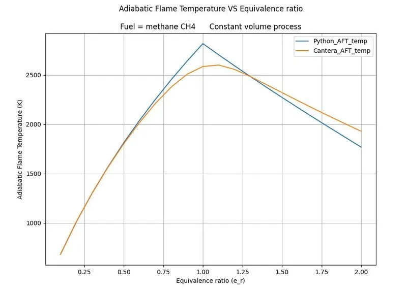
- As the Equivalence(e_r) ratio increases from 0 to 1 AFT also increases because er < 1 means lean mixture. there is no enough air to complete the 100% combustion.
- at er = 1 fuel gets completely burnt gives maximum temperature. if e_r value increased beyond 1 => e_r > 1, means rich mixture of excess fuel absorbs heat and the AFT temperature reduces if we increase e_r value after Stoichiometry combustion.
- The temperatures obtained by using the numerical program and by using the Cantera module are closer and almost the same when e_r is in between 0-0.5. when e_r > 0.5 the AFT temperatures are diverging because Cantera uses a chemical kinematics library so it predicts more accurate product composition means more number of species than the species that we considered in the numerical calculation.
2) Adiabatic flame temperature variation with Heat loss (In constant pressure-chamber) :
Consider a constant pressure reactor with heat loss. The reactor is initially set at STP conditions.
The heat loss should be input in your program and must be a fraction of the "maximum possible heat loss".
Find the AFT of CH4 with H_loss = 0.35
maximum possible heat loss = `m_f * LHV`
fuel =CH4
`"mass of fuel"=m_f = 16.04e-3 (Kg)/(mol)`
`"Lower Heating Value"=LHV =50e6 J/(Kg)`
Procedure:
- import math, Numpy, Matplotlib.pyplot & Cantera libraries as modules.
- Writing a function to calculate the enthalpy of Reactance and Products using NASA Polynomial by taking temperature and Species coefficients as inputs.`H/(R*T)=a1+a2*(T/2)+a3*(T^2/3)+a4*(T^3/4)+a5*(T^4/5)+(a6)/T`
- Define the lower and higher temperature Coefficients of Reactance and Product species according to the side of involvement.
- Writing a function that calculates `H_("react")-H_("prod")+H_("loss")*Q_(max)` by taking temperature and Heat loss coefficient as inputs.
- Writing a function to calculate the 2nd order numerical derivative of the above function using the Foward differencing approach.
- Setting a for loop to calculate AFT for various Heat loss coefficients.
- In the for loop set a while loop to perform the Newton Raphson root finding method to calculate AFT for each Heat loss coefficient.
- plot the results.
# Adiabatic flame temperature variation with Heat loss
# (In constant Pressure-chamber) :

# in this program we are going to calculate the AFT of Methane at different hear loss values at equalance ratio = 1

import math
import matplotlib.pyplot as plt
import numpy as np

def h(T,co_eff):

	R  = 8.314 #j/mol-K
	a1 = co_eff[0]
	a2 = co_eff[1]
	a3 = co_eff[2]
	a4 = co_eff[3]
	a5 = co_eff[4]
	a6 = co_eff[5]
	return R*T*(a1 + a2*T/2 + a3*pow(T,2)/3 + a4*pow(T,3)/4 + a5*pow(T,4)/5 + a6/T)

CH4_coeff_l = [5.14987613E+00, -1.36709788E-02, 4.91800599E-05, -4.84743026E-08, 1.66693956E-11, -1.02466476E+04]
O2_coeff_l  = [3.78245636E+00, -2.99673416E-03, 9.84730201E-06, -9.68129509E-09, 3.24372837E-12, -1.06394356E+03]
N2_coeff_l  = [0.03298677E+02, 0.14082404E-02, -0.03963222E-04, 0.05641515E-07, -0.02444854E-10, -0.10208999E+04]

CO2_coeff_h = [3.85746029E+00, 4.41437026E-03, -2.21481404E-06, 5.23490188E-10, -4.72084164E-14, -4.87591660E+04]
H20_coeff_h = [3.03399249E+00, 2.17691804E-03, -1.64072518E-07, -9.70419870E-11, 1.68200992E-14, -3.00042971E+04]
N2_coeff_h  = [0.02926640E+02, 0.14879768E-02, -0.05684760E-05, 0.10097038E-09, -0.06753351E-13, -0.09227977E+04]

def G(T,H_loss_percent,Q):
	# Roots finding problem
	T_stp    = 298.15          #STP
	# Enthalpy of Reactance
	h_CH4_r = h(T_stp,CH4_coeff_l)
	h_O2_r  = h(T_stp,O2_coeff_l)
	h_N2_r  = h(T_stp,N2_coeff_l)
	H_reactance = h_CH4_r + 2*(h_O2_r + 3.76*h_N2_r)

	# Enthalpy of Products
	h_CO2_p = h(T,CO2_coeff_h)
	h_H20_p = h(T,H20_coeff_h)
	h_N2_p  = h(T,N2_coeff_h)
	H_products = h_CO2_p + 2*h_H20_p + 7.52*h_N2_p

	return (H_products - H_reactance)  + H_loss_percent*Q

def Gprime(T,H_loss_percent,Q):
	return (G(T+1e-6,H_loss_percent,Q)-G(T,H_loss_percent,Q))/1e-6

# Heat loss calculation
mass_CH4 = 16.04e-3   # kg/mol
HHV_CH4  = 55.5e6     # J/Kg
LHV_CH4  = 50.0e6     # J/Kg
max_Q_loss = Q = LHV_CH4*mass_CH4
#print(max_Q_loss)

alpha   = 0.2
tol     = 1e-3
H_loss_percentages  = np.linspace(0.05,1,20)
print(type(H_loss_percentages))
print((H_loss_percentages))
AFT_temp = []

for H_loss_percent in H_loss_percentages:
	T_guess = 1500
	itr     = 0
	while (abs(G(T_guess,H_loss_percent,Q)) > tol):
		T_guess = T_guess - alpha*(G(T_guess,H_loss_percent,Q)/Gprime(T_guess,H_loss_percent,Q))
		itr = itr + 1
		if H_loss_percent == 0.35:
			plt.plot(itr,T_guess,'*',color='blue')
			plt.xlabel('iterations')
			plt.ylabel('Adiabatic Flame temperature K')
			plt.title('Adiabatic Flame temperature VS iterations \n heat loss coefficient = 0.35')
			plt.grid('on')
	AFT_temp.append(T_guess)

#print(AFT_temp)

#H_loss_35 = np.where(H_loss_percentages==0.35)
H_loss_35 = np.searchsorted(H_loss_percentages, 0.35)    # finding index
AFT_temp_35 = AFT_temp[H_loss_35]                        # AFT temperature with 35% heat loss
print('Adiabatic Flame Temperature of methane CH4 with 35 percent of Heatloss :', AFT_temp_35)

plt.figure(2)
plt.plot(H_loss_percentages,AFT_temp)
plt.xlabel('Heat loss Percentage (coefficient)')
plt.ylabel('Adiabatic Flame temperature K')
plt.title('Adiabatic Flame temperature VS Heat loss coefficient')
plt.grid('on')
plt.show()
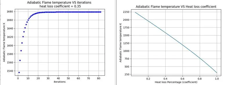
Adiabatic Flame Temperature of methane CH4 with 35 percent of Heat loss: 1678.8363912616562 K
Conclusion:
- As the Heat loss coefficient increases indicate more Heat rejection leads to a decrease in AFT temperature, AFT maximum at Heat loss coefficient= 0, AFT = T_stp when Heat loss coefficient = 1.
- As the number of iterations increases Newton's Raphson method predicts more accurate results.
- Adiabatic Flame Temperature of methane CH4 with 35 percent of Heat loss: 1678.8363912616562 K
3) Adiabatic flame temperature variation with respect to Alkane, Alkene, Alkyne :
Test it only for Alkane, Alkene & Alkyne variants of 2 Carbon atom chain and plot a trend.
Assume no heat loss.
Alkanes CnH2n+2
Alkenes CnH2n.
alkynes CnH2n-2.
number of carbon atoms n = 2
Ethane = C2H6, Ethylene = C2H4,& Acetylene = C2H2
The procedure is the same as the constant pressure-chamber AFT calculation expect Heat loss.
in this AFT is calculated for 3 different Alkane, Alkene, Alkyne fuels and comparing with Cantera results.
# Adiabatic flame temperature variation with respect to Alkane, Alkene, Alkyne
# in this program we are going to calculate the AFT of Ethane, Ethylene,& Acetylene
# Alkanes  CnH2n+2
# Alkenes  CnH2n.
# alkynes  CnH2n-2.
# number of carbon atoms n = 2
# Ethane = C2H6, Ethylene = C2H4,& Acetylene = C2H2
#  stoichiometric reaction
# CxHy + (x+y/4)(O2+3.76N2) = x*CO2 + y/2*H2O + (x+y/4)*7.52*N2

import math
import matplotlib.pyplot as plt
import numpy as np
import cantera as ct

def h(T,co_eff):

	R  = 8.314 #j/mol-K
	a1 = co_eff[0]
	a2 = co_eff[1]
	a3 = co_eff[2]
	a4 = co_eff[3]
	a5 = co_eff[4]
	a6 = co_eff[5]
	return R*T*(a1 + a2*T/2 + a3*pow(T,2)/3 + a4*pow(T,3)/4 + a5*pow(T,4)/5 + a6/T)

# low temperrture coefficients of reactance
C2H6_coeff_l = [4.29142492E+00, -5.50154270E-03, 5.99438288E-05, -7.08466285E-08, 2.68685771E-11,-1.15222055E+04]
C2H4_coeff_l = [3.95920148E+00, -7.57052247E-03, 5.70990292E-05, -6.91588753E-08, 2.69884373E-11, 5.08977593E+03]
C2H2_coeff_l = [8.08681094E-01, 2.33615629E-02, -3.55171815E-05, 2.80152437E-08, -8.50072974E-12, 2.64289807E+04]

O2_coeff_l  = [3.78245636E+00, -2.99673416E-03, 9.84730201E-06, -9.68129509E-09, 3.24372837E-12, -1.06394356E+03]
N2_coeff_l  = [0.03298677E+02, 0.14082404E-02, -0.03963222E-04, 0.05641515E-07, -0.02444854E-10, -0.10208999E+04]

# High temperature coefficients of productus
CO2_coeff_h = [3.85746029E+00, 4.41437026E-03, -2.21481404E-06, 5.23490188E-10, -4.72084164E-14, -4.87591660E+04]
H20_coeff_h = [3.03399249E+00, 2.17691804E-03, -1.64072518E-07, -9.70419870E-11, 1.68200992E-14, -3.00042971E+04]
N2_coeff_h  = [0.02926640E+02, 0.14879768E-02, -0.05684760E-05, 0.10097038E-09, -0.06753351E-13, -0.09227977E+04]

def solution(fuel_Enthalpy,x,y,h_O2_r,h_N2_r,h_CO2_p,h_H20_p,h_N2_p):
	# CxHy + (x+y/4)(O2+3.76N2) = x*CO2 + y/2*H2O + (x+y/4)*7.52*N2
	H_reactance = fuel_Enthalpy + (x + y/4)*(h_O2_r + 3.76*h_N2_r)
	H_products  = x*h_CO2_p + (y/2)*h_H20_p + (x + y/4)*3.76*h_N2_p
	return (H_products - H_reactance)

def G(T,Hydrocarbon):
	# Roots finding problem
	R_u = 8.3144  # universal gas constant J/molK

	T_stp    = 298.15            #STP
	# Enthalpy of Reactance
	h_C2H6_r = h(T_stp,C2H6_coeff_l)
	h_C2H4_r = h(T_stp,C2H4_coeff_l)
	h_C2H2_r = h(T_stp,C2H2_coeff_l)
	h_O2_r  = h(T_stp,O2_coeff_l)
	h_N2_r  = h(T_stp,N2_coeff_l)

	# Enthalpy of Products
	h_CO2_p = h(T,CO2_coeff_h)
	h_H20_p = h(T,H20_coeff_h)
	h_N2_p  = h(T,N2_coeff_h)

	React_Prod_array = [h_O2_r,h_N2_r,h_CO2_p,h_H20_p,h_N2_p]

	if Hydrocarbon == 'Alkane':
		# Alkanes  CnH2n+2 = CxHy = C2H6 =Ethane
		x, y = 2,6
		H_net = solution(h_C2H6_r,x,y,*React_Prod_array)
	elif Hydrocarbon == 'Alkene':
		#Alkenes  CnH2n = CxHy = C2H4 = Ethylene
		x, y = 2,4
		H_net = solution(h_C2H4_r,x,y,*React_Prod_array)
	elif Hydrocarbon == 'Alkyne':
		#Alkynes  CnH2n-2 = CxHy = C2H2 = Acetylene
		x, y = 2,2
		H_net = solution(h_C2H2_r,x,y,*React_Prod_array)

	return H_net

def Gprime(T,Hydrocarbon):
	# Numerical derivative of function (Forward differencinf)
	return (G(T+1e-6,Hydrocarbon)-G(T,Hydrocarbon))/1e-6

Hydrocarbons = ['Alkane', 'Alkene', 'Alkyne']
alpha   = 0.1
tol     = 1e-3
AFT_temperature_python = []

for Hydrocarbon in Hydrocarbons:
	T_guess = 1900
	while (abs(G(T_guess,Hydrocarbon)) > tol):
		T_guess = T_guess - alpha*(G(T_guess,Hydrocarbon)/Gprime(T_guess,Hydrocarbon))

	AFT_temperature_python.append(T_guess)


# AFT Calculation using Cantera
gas = ct.Solution('gri30.xml')
species = ['C2H6','C2H4','C2H2']
a = [3.5,3,2.5]
AFT_temperature_cantera  = []

for i in range(3):
	gas.TPX = 298.15, 101325,{species[i] :1, 'O2' :a[i], 'N2' :a[i]*3.76}   # Get/Set temperature [K], pressure [Pa], and mole fractions.
	gas.equilibrate('HP','auto')
	#auto =The element potential solver will be tried first, then if it fails the Gibbs solver will be tried.
	#UV = Get/Set internal energy [J/kg or J/kmol] and specific volume[m^3/kg or m^3/kmol]
	AFT_temperature_cantera.append(gas.T)

AFT_Temp = [AFT_temperature_python,AFT_temperature_cantera]

# plotting results
for i in range(3):
	plt.bar(Hydrocarbons[i],AFT_temperature_python[i],color='r')
	plt.bar(species[i],AFT_temperature_cantera[i],color='g')
plt.ylabel('Adiabatic Flame Temperature (K)')
plt.title('''Adiabatic flame temperature variation of Alkane, Alkene, Alkyne  fuels in \n
	using Python & Cantera''')
plt.legend(['AFT temperature using python','AFT temperature using Cantera'],loc='lower right')
plt.show()

print(AFT_temperature_cantera)
print(AFT_temperature_python)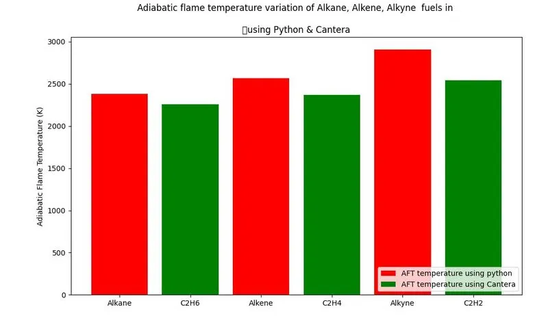
Conclusions:
- For Alkane, Alkene & Alkyne variants (Ethane = C2H6, Ethylene = C2H4,& Acetylene = C2H2)of 2 Carbon atom chain have a same number of carbon atoms but a different number of hydrogen atoms, as the number of hydrogen atoms increases leads to decrease in the AFT temperature because hydrogen in reactance leads to produce water H2O on the products side. more hydrogen on the reactance side more water on the products side.
- Cantera AFT temperatures are lower than python AFT temperatures because Cantera uses more species on the product side.
4) Adiabatic flame temperature variation with respect to a number of Carbon atom chains :
For a general alkane, plot the effect of the number of carbon atoms (from 1 to 3) on the final temperature. Assume no heat loss.
For a general alkane
Alkanes CnH2n+2 where n = number of carbon atoms (n = 1,2,3)
n = 1: methane = CH4
n = 2: ethane = C2H6
n = 3: propane = C3H8
The procedure is same as the constant pressure-chamber AFT calculation expect Heat loss.
in this AFT is calculated for 3 different n values of Alkane fuels and comparing with Cantera results.
# Adiabatic flame temperature variation with respect to a number of Carbon atom chains :
# For a general alkane
# Alkanes  CnH2n+2 where n = number of carbon atoms (n = 1,2,3)
# n = 1: methane = CH4
# n = 2: ethane  = C2H6
# n = 3: propane = C3H8
#  stoichiometric reaction
# CxHy + (x+y/4)(O2+3.76N2) = x*CO2 + y/2*H2O + (x+y/4)*7.52*N2

import math
import matplotlib.pyplot as plt
import numpy as np
import cantera as ct

def h(T,co_eff):

	R  = 8.314 #j/mol-K
	a1 = co_eff[0]
	a2 = co_eff[1]
	a3 = co_eff[2]
	a4 = co_eff[3]
	a5 = co_eff[4]
	a6 = co_eff[5]
	return R*T*(a1 + a2*T/2 + a3*pow(T,2)/3 + a4*pow(T,3)/4 + a5*pow(T,4)/5 + a6/T)

# low temperrture coefficients of reactance
CH4_coeff_l  = [5.14987613E+00, -1.36709788E-02, 4.91800599E-05, -4.84743026E-08, 1.66693956E-11, -1.02466476E+04]
C2H6_coeff_l = [4.29142492E+00, -5.50154270E-03, 5.99438288E-05, -7.08466285E-08, 2.68685771E-11, -1.15222055E+04]
C3H8_coeff_l = [0.93355381E+00,  0.26424579E-01, 0.61059727E-05, -0.21977499E-07, 0.95149253E-11, -0.13958520E+05]

O2_coeff_l  = [3.78245636E+00, -2.99673416E-03, 9.84730201E-06, -9.68129509E-09, 3.24372837E-12, -1.06394356E+03]
N2_coeff_l  = [0.03298677E+02, 0.14082404E-02, -0.03963222E-04, 0.05641515E-07, -0.02444854E-10, -0.10208999E+04]

# High temperature coefficients of productus
CO2_coeff_h = [3.85746029E+00, 4.41437026E-03, -2.21481404E-06, 5.23490188E-10, -4.72084164E-14, -4.87591660E+04]
H20_coeff_h = [3.03399249E+00, 2.17691804E-03, -1.64072518E-07, -9.70419870E-11, 1.68200992E-14, -3.00042971E+04]
N2_coeff_h  = [0.02926640E+02, 0.14879768E-02, -0.05684760E-05, 0.10097038E-09, -0.06753351E-13, -0.09227977E+04]

def solution(fuel_Enthalpy,x,y,h_O2_r,h_N2_r,h_CO2_p,h_H20_p,h_N2_p):
	# CxHy + (x+y/4)(O2+3.76N2) = x*CO2 + y/2*H2O + (x+y/4)*7.52*N2
	H_reactance = fuel_Enthalpy + (x + y/4)*(h_O2_r + 3.76*h_N2_r)
	H_products  = x*h_CO2_p + (y/2)*h_H20_p + (x + y/4)*3.76*h_N2_p
	return (H_products - H_reactance)

def G(T,Alkane):
	# Roots finding problem
	R_u = 8.3144  # universal gas constant J/molK

	T_stp    = 298.15            #STP
	# Enthalpy of Reactance
	h_CH4_r = h(T_stp,CH4_coeff_l)
	h_C2H6_r = h(T_stp,C2H6_coeff_l)
	h_C3H8_r = h(T_stp,C3H8_coeff_l)
	h_O2_r  = h(T_stp,O2_coeff_l)
	h_N2_r  = h(T_stp,N2_coeff_l)

	# Enthalpy of Products
	h_CO2_p = h(T,CO2_coeff_h)
	h_H20_p = h(T,H20_coeff_h)
	h_N2_p  = h(T,N2_coeff_h)

	React_Prod_array = [h_O2_r,h_N2_r,h_CO2_p,h_H20_p,h_N2_p]

	if Alkane == 'methane':
		# Alkanes  CnH2n+2 = CxHy = CH4 = methane
		x, y = 1,4
		H_net = solution(h_CH4_r,x,y,*React_Prod_array)
	elif Alkane == 'ethane':
		# Alkanes  CnH2n+2 = CxHy = C2H6 = Ethane
		x, y = 2,6
		H_net = solution(h_C2H6_r,x,y,*React_Prod_array)
	elif Alkane == 'propane':
		# Alkanes  CnH2n+2 = CxHy = C3H8 = propane
		x, y = 3,8
		H_net = solution(h_C3H8_r,x,y,*React_Prod_array)

	return H_net

def Gprime(T,Alkane):
	# Numerical derivative of function (Forward differencinf)
	return (G(T+1e-6,Alkane)-G(T,Alkane))/1e-6

Alkanes = ['methane', 'ethane', 'propane']
alpha   = 0.9
tol     = 1e-3
AFT_temperature_python = []

for Alkane in Alkanes:
	T_guess = 1500
	while (abs(G(T_guess,Alkane)) > tol):
		T_guess = T_guess - alpha*(G(T_guess,Alkane)/Gprime(T_guess,Alkane))

	AFT_temperature_python.append(T_guess)


# AFT Calculation using Cantera
gas = ct.Solution('gri30.xml')
species = ['CH4','C2H6','C3H8']
a = [2,3.5,5]
AFT_temperature_cantera  = []

for i in range(3):
	gas.TPX = 298.15, 101325,{species[i] :1, 'O2' :a[i], 'N2' :a[i]*3.76}
	gas.equilibrate('HP','auto')
	AFT_temperature_cantera.append(gas.T)

AFT_Temp = [AFT_temperature_python,AFT_temperature_cantera]

# plotting results
for i in range(3):
	plt.bar(Alkanes[i],AFT_temperature_python[i],color='r')
	plt.bar(species[i],AFT_temperature_cantera[i],color='g')
plt.ylabel('Adiabatic Flame Temperature (K)')
plt.title('''Adiabatic flame temperature variation with respect to a number of Carbon atom chains :
	For a general alkane fuels  methane, ethane & propane\n
	using python and cantera''')
plt.legend(['AFT temperature using python','AFT temperature using Cantera'],loc='lower right')
plt.show()

print(AFT_temperature_cantera)
print(AFT_temperature_python)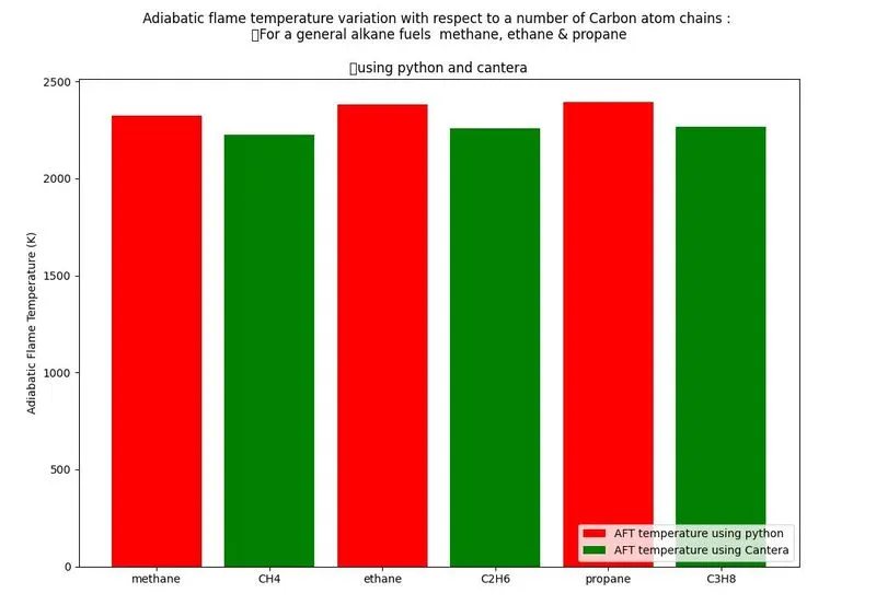
Conclusions:
- For general Alkanes (CnH2n+2) of the number of carbon atoms (from 1 to 3) (methane = CH4, ethane = C2H6, propane = C3H8), as the number of carbon atoms increase leads to an increase in the AFT temperature, because more carbon in reactance leads to produce more Heat. more Heat leads to an increase in AFT temperature.
- Cantera AFT temperatures are lower than python AFT temperatures because Cantera uses more species on the product side.