Week 3 - Adiabatic Flame Temperature calculation
Adiabatic Flame Temperature calculation
Aim:
The main objective of this challenge is to calucculate the Adiabatic Falme Temperature for given conditions using Python and Cantera.
Adiabatic Flame Temperature:
The adiabatic flame temperature (AFT) is defined as the temperature attained when all of the chemical reaction heat released by heating combustion products. The adiabatic flame temperature is one that occurs when the combustion chamber is well insulated with no heat losses (adiabatic conditions). The peak adiabatic flame temperature occurs at around Φ = 1 in an ideally insulated combustion chamber. As percent combustion air increases, that is, as we deviate from the stoichiometric condition, some of the heat generated is used to heat up the excess air. As a result, the flame temperature will drop.
Therefore, under controlled conditions, flame temperature can be a useful measure of air-fuel ratio, that is, how far we deviate from stoichiometric conditions and whether the combustion is fuel-lean or fuel-rich. Note that although we have illustrated flame temperature with stoichiometric air (100%), the same general rules apply to any combustion condition. This is helpful because it allows temperature control by changing the air-fuel mixture. It also gives us a sense of whether unburned fuel is being released into the atmosphere. In order to maintain the flame temperature at any set of conditions, one must increase or decrease the fuel and air proportionately. Increasing fuel alone or air alone will result in a change in flame temperature.
In the study of combustion, there are two types of adiabatic flame temperature depending on how the process is completed: the constant volume and constant pressure; both of which describe temperature that combustion products theoretically can reach if no energy is lost to the outside environment.
For any process, we know the reactants are at room temperature. To find the adiabatic flame temperature, we will use Newton Raphson method with a guess temperature and by iterating the defined function with the derivative function.
The newton raphson method is an iterative method used to find the root of a function f(x) with an initial guess and iterating it to the solution becomes to zero.

Conditions at which we have to caluculate the Adibatic Flame Temperature:
1. Adiabatic flame temperature variation with Equivalence ratio (In constant volume-chamber) :
2. Adiabatic flame temperature variation with Heat loss (In constant pressure-chamber) :
3. Adiabatic flame temperature variation with respect to Alkane, Alkene, Alkyne :
4. Adiabatic flame temperature variation with respect to a number of Carbon atom chains :
Adibatic Flame Temperature at constant volume combustion by varying the equivalence ratio:
Before going into the theory of the Adibatic Flame Temperature at constant volume combustion, let us discuss about equivalence ratio.
The equivalence ratio is defined as the ratio of the actual fuel/air ratio to the stoichiometric fuel/air ratio. Stoichiometric combustion occurs when all the oxygen is consumed in the reaction, and there is no molecular oxygen(O2) in the products.
Equivalence ratio, Φ = (A/F)actual/(A/F) stoichometric
If the equivalence ratio (phi) is equal to one, the combustion is stoichiometric. If phi is < 1, the combustion is lean with excess air, and if phi is >1, the combustion is rich with incomplete combustion.
Generic formula for Methane with oxygen and nitrogen:
CxHy + a(O2 + 3.76N2) = xCO2 + (y/2)H2O + 3.76aN2.
If the combustion takes place at lean or stoichometric Condition: (Φ <= 1):
As the mixture is at lean or Stoichometric conditions, the product species are very similar to the generic reaction, and balancing the chemical reaction is also simple.
CxHy + a(O2 + 3.76N2) = bCO2 + dH2O + fO2 + 3.76aN2.
Where, (x,y),a,b,d,f indicates the number of moles of that species. These are caluculated by equating at both sides which are as follows:
a = (x + (y/4))/Φ
b = x
d = y/2
f = ((1-Φ))/Φ*(x + y/4)
If the combustion takes place at rich Condition: (Φ > 1):
As the fuel is at rich condition which means of more carbon atoms which has more chance to form CO by dissasociating with H2O and forming the reaction as follows. Balancing the reaction involves huge caluculations because of involvement of more species.
CxHy + a(O2 + 3.76N2) = bCO2 + cCO + dH2O + eH2 + 3.76aN2.
The mole fractions of each species is caluculated as follows:
a = (x + (y/4))/phi
kp = 0.3754 * (T**(-0.719))
b =( (2*a*(kp - 1) + x + (y/2))/2*(kp - 1))*((2*a*(kp - 1) + x + (y/2))**2) - 4*kp*(kp - 1)*(2*a*x -x**2))^1/2
c = x - b
d = 2*a - b - x
e = -2*a + b + x+ (y/2)
As we got to know about equivalence ratio, at constant Volume combustion, the Adiabatic Flame Temperature is caluculated as follows:
If the combustion happens adiabatically at constant Volume, we know it will increase the internal enery of the system. The adiabatic flame temperature is caluculated by equating the internal energies of the reactants and products. From first law of thermodyanamics,
delQ - delW = delU
As the combustion is taking place at adiabatic conditons,
delQ = 0.
Work done, W = pdv,
As the system is at constant volume dv = 0 which results in delw = 0,
delU=0
Upr -Ure = 0
Ure (Pi, Vi) = Upr (Pf, Vf)
Since most of the thermodyanamic properties provides values for enthalpy (H) rather than internal energy, the above equation becomes:
We know internal energy is a function of enthalpy and volume at constant pressure.
H = U + pV
U = H - PV
Because we are caluculating in terms of enthlapy
(H-pV)pr = (H-pV)re
pV = NRT
Hre - Hpr -(Nre*Ru*Tstp - Npr*Ru*Tad) = 0
Before writing the code in python, to find the values of enthalpies of different species at different temperature. We are using NASA polynomial function as follows:
H(T) =(a1 + a2*T/2 + a3*pow(T,2)/3 + a4*pow(T,3)/4 + a5*pow(T,4)/5 + a6/T)*R*T
Where ai are the coeffiecients of each species, the values for these are imported form the GRI -MECH thermodynamic .dat file. If the temperature is above 1000k, then we will consider the coefficients of first seven values and if the temperature is above 350 and below 1000k, we have to use the later seven values.
CODE SNIPPET FOR CASE I:
"""
Caluculating adiabatic flame temperature at constant volume
internal energy of products = internal energy of reactants
Upr = Ure
H = U + pV
U = H - PV
(H-pV)pr = (H-pV)re       #Because we are caluculating in terms of enthlapy
pV = NRT
Hre - Hpr -(Nre*Ru*Tstp - Npr*Ru*Tad)
Considering Methane and air for this combustion.
CxHy+a(O2+3.56N2) = bCo2 +cCO + dH2O + eH2 + fO2 + 3.76aN2

"""

import matplotlib.pyplot as plt
import math
import numpy as np

"""
We know kFT is caluculated by subracting the enthalpies of products with reactants
"""
#univaersal gas constant
R = 8.314 #J/mol-K

#Function to return the values of enthalpies in joule/mol for each species:

def h(T,co_effs):
	k = co_effs

	return (k[0] + k[1]*T/2 + k[2]*pow(T,2)/3 + k[3]*pow(T,3)/4 + k[4]*pow(T,4)/5 + k[5]/T)*R*T

#low temperature coefficients (T<=1000k)
ch4_coeffs_l = [5.14987613E+00, -1.36709788E-02, 4.91800599E-05, -4.84743026E-08, 1.66693956E-11, -1.02466476E+04,-4.64130376E+00]
o2_coeffs_l  = [3.78245636E+00, -2.99673416E-03, 9.84730201E-06, -9.68129509E-09, 3.24372837E-12, -1.06394356E+03, 3.65767573E+00]
n2_coeffs_l  = [0.03298677E+02, 0.14082404E-02, -0.03963222E-04, 0.05641515E-07, -0.02444854E-10, -0.10208999E+04, 0.03950372E+02]

#low temperature coefficients  (T>1000k)
co2_coeffs_h = [3.85746029E+00, 4.41437026E-03, -2.21481404E-06, 5.23490188E-10, -4.72084164E-14, -4.87591660E+04, 2.27163806E+00]
co_coeffs_h  = [2.71518561E+00, 2.06252743E-03, -9.98825771E-07, 2.30053008E-10, -2.03647716E-14, -1.41518724E+04, 7.81868772E+00]
h2o_coeffs_h = [3.03399249E+00, 2.17691804E-03, -1.64072518E-07, -9.70419870E-11, 1.68200992E-14, -3.00042971E+04, 4.96677010E+00]
h2_coeffs_h  = [3.33727920E+00, -4.94024731E-05, 4.99456778E-07, -1.79566394E-10, 2.00255376E-14, -9.50158922E+02,-3.20502331E+00]
o2_coeffs_h  = [3.78245636E+00, -2.99673416E-03, 9.84730201E-06, -9.68129509E-09, 3.24372837E-12, -1.06394356E+03, 3.65767573E+00]
n2_coeffs_h  = [0.02926640E+02, 0.14879768E-02, -0.05684760E-05, 0.10097038E-09, -0.06753351E-13, -0.09227977E+04, 0.05980528E+02]


#Function to return the values of enthalpies at given temperature at Constant volume combustion:
def f(T,phi):

	x = 1
	y = 4

	if phi<=1:
		#If the equivalance ratio is less than it is lean mixture and euqual to one, it is called stoichometric mixture
		#CxHy+a(O2+3.56N2) = bCo2 + dH2O + fO2 + 3.76aN2
		a = (x + (y/4))/phi
		b = x
		c = 0
		d = y/2
		e = 0
		f = ((1-phi))/phi*(x + y/4)

	if phi>1:
		#If the equivalence ratio is greater than one, it is calld rich mixture
		#CxHy+a(O2+3.56N2) = bCo2 +cCO + dH2O + eH2 + 3.76aN2
		a = (x + (y/4))/phi
		kp = 0.3754 * (T**(-0.719))
		b = (2*a*(kp - 1) + x + (y/2))/2*(kp - 1)
		p = (2*a*(kp - 1) + x + (y/2))**2
		q = 4*kp*(kp - 1)*(2*a*x -x**2)
		b = b - (1/(2*(kp - 1)))*(p - q)**0.5
		c = x - b
		d = 2*a - b - x
		e = -2*a + b + x+ (y/2)
		f = 0


	Tstp = 298.15  #k
	h_ch4_r = h(Tstp,ch4_coeffs_l)
	h_o2_r  = h(Tstp,o2_coeffs_l)
	h_n2_r  = h(Tstp,n2_coeffs_l)

	#CxHy+a(O2+3.56N2)
	H_reactants = h_ch4_r + (2/phi)*h_o2_r + (7.52/phi)*h_n2_r
	NRT_reactants = (1 + (2/phi) + (7.52/phi))*R*Tstp

	#caluculating enthalpies of each species of reactants at given temperature:
	h_co2_p = h(T, co2_coeffs_h)
	h_co_p  = h(T, co_coeffs_h)
	h_h2o_p = h(T, h2o_coeffs_h)
	h_h2_p  = h(T, h2_coeffs_h)
	h_o2_p  = h(T, o2_coeffs_h)
	h_n2_p  = h(T, n2_coeffs_h)

	#bCo2 +cCO + dH2O + eH2 + fO2 + 3.76aN2

	H_products = b*h_co2_p + c*h_co_p + d*h_h2o_p + e*h_h2_p + f*h_o2_p + 3.76*a*h_n2_p
	NRT_products = (b + c + d + e + f + 3.76*a)*R*T

	return(H_reactants - H_products) - (NRT_reactants - NRT_products)


#defining a derivative of the above function, Considering forward differencing method:  (f(x+dx)-f(x))/dx)

def fprime(T,phi):
	return(f(T+1e-6, phi)-f(T, phi))/1e-6            # dT = 1e-6

# Creating the phi values with combination of lean and rich mixtures
#As the values are of float, we are using numpy to create an array

phi = np.arange(0.6,1.55,0.05)     #starting value, ending value, step in between
print(phi)

#creating a null list of the adiabatic flame temparature
AFT_py = []
for i in range(len(phi)):
	T_guess = 1500
	alpha = 0.5              #relaxation factor
	tol = 1e-3               #tolerance
	ct = 1					 # iteration counter
	while(abs(f(T_guess, phi[i])) >= tol):
		T_guess = T_guess-((f(T_guess, phi[i])/fprime(T_guess, phi[i])))*alpha
		ct = ct+1
	AFT_py.append(T_guess)              # adding each value of AFT to the list created earlier.

print(ct)
print(AFT_py)


# Caluculating the AFT values using Cantera:
import cantera as ct
gas = ct.Solution('gri30.xml')
AFT_ct = []

for i in range(0,len(phi)):

	gas.TPX = 298.15,101325,{'CH4':1, 'O2':2/phi[i], 'N2':7.52/phi[i]}
	gas.equilibrate('UV','auto')
	AFT_ct.append(gas.T)

print(AFT_ct)

#plotting the graphs
plt.plot(phi,AFT_py,'-o',color='blue', label='Python')
plt.plot(phi,AFT_ct,'-s',color='green', label='Cantera')
plt.xlabel('Equivalence Ratio ($Phi$)')
plt.ylabel('Adiabatic Flame Temperature (K)')
plt.grid('on')
plt.minorticks_on()
plt.title('Adiabatic Flame Temperature (vs) Equivalence Ratio \n Methane-Air Combustion at Constant volume', fontsize = 12)
plt.legend(fontsize = 12)
plt.show()


#To create the resulted values in a  tabular form
from prettytable import PrettyTable as PT
x = phi
y = AFT_py
z = AFT_ct

table = PT(['phi', 'AFT_py', 'AFT_ct'])
for i in range(0,len(phi)):
	table.add_row([x[i],y[i],z[i]])

print(table)
Procedure:
- As mentioned in the theory, we copy the values for the co-efficients for the reactants at low temperature and products with high temperature which makes sense.
- We have to define a function for enthalpy(h) for each species with these coefficients and temperature.
- Next we will define a function for caluculating the enthalpy (H) for all reactants(at STP which is known) and products(at AFT which is unknown) by using the above function and at the end equating the difference with zero.
- But we need to find the AFT for different values of Phi, so as per thoery using if function defining all the values for mole fractions.
- By using a set of values of phi and defining a derivative for the above function using forward differencing method.
- Using newton raphson method, we will iterate to find the value for Adiabatic flame temperature by varying the phi values using a for loop.
- After that using Cantera, we will using the GRI MECH30.xml file to find the solution.
- By using the 'UV' function we will define the temperature, pressure and mole fractions of each reactant in a dictionary, printing the values of AFT by varying the Phi values usnig for loop.
- PLotting the values of AFT caluculated from python and cantera.
RESULTS:
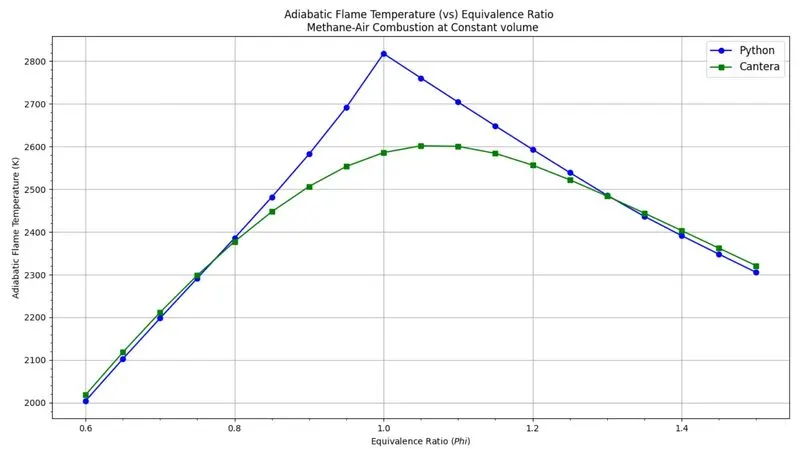
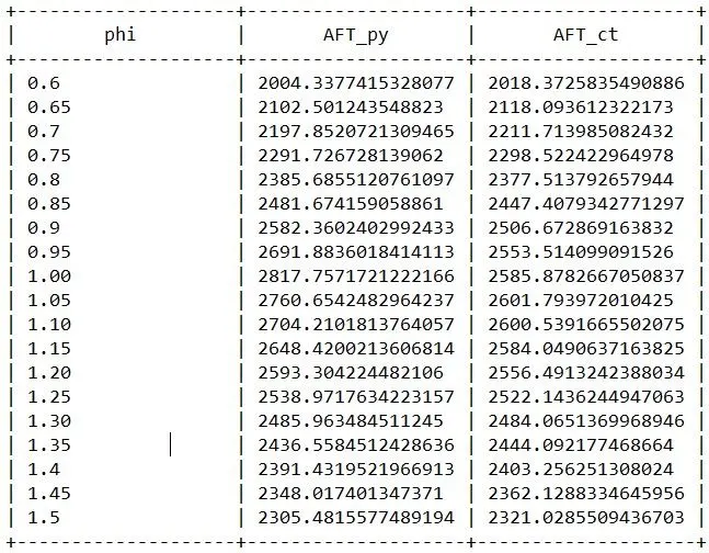
The values are tabulated as follows:
OBSERVATION:
- We can observe the highest temperature recorded for theoritical caluculation from python at phi = 1, this is because in theoritical caluculations we only consider some species in products. But in practical, lot of species resluts from combustion which is consider in Cantera, which utilises the temperature.
- Another thing we can observe form the above plot and table is for both theoritical and cantera caluculations, the highest temperature is recorded at range of phi = 1.0 to 1.05. The main reason behind it is that only at this condition the fuel gets complete oxidization which results in complete combustion .
- And the important point I have observed form the above plot is that at intial stage at Φ = 0.5, indicates the fuel-lean system in which hydrocarbon size is small and the oxidizer is high which results in forming low temperature. Similarly at Φ = 1.5, as the size of the hydrocarbon is high, it forms negative heat energy because of less oxidization which results in forming of CO2 and H2, CO species in the prodcuts which utilises the temperature. So the curve starts form low temperature and raises at Φ = 1, and again starts to drop when the equivalence ratio is increasing.
Adiabatic flame temperature variation with Heat loss at Constant pressure combustion:
As we know adiabatic flame temperature helps us to know the highest temperatue results from the combustion, so that we can design our system accordingly. But in caluculating this we considering the combustion is taking place at adiabatic conditions, where in practical conditions it is not possible. A definite amount of heat loss will occur is some situations, we have to consider that loss also to get an exact value of highest tempertaure.
For that we are considering the system at constant pressure to capture the results with heat loss. From first law of thermodyanamics,
delQ - delW = delU
As the combustion is taking place at adiabatic conditons,
delQ = 0.
Work done, W = pdv,
As the system is at constant pressure,
-p(Vf - Vi) = Uf - Ui,
Ui+P*Vi = Uf + P* Vf, (H= U+PV)
Hre = Hpr.
Considering Heat loss with low heating value,
Hpr- Hre+hloss(LHV) = 0
Why considering low heating value?
The lower heating value (also known as net calorific value) of a fuel is defined as the amount of heat released by combusting a specified quantity (initially at 25°C) and returning the temperature of the combustion products to 150°C, which assumes the latent heat of vaporization of water in the reaction products is not recovered.
The higher heating value (also known gross calorific value or gross energy) of a fuel is defined as the amount of heat released by a specified quantity (initially at 25°C) once it is combusted and the products have returned to a temperature of 25°C, which takes into account the latent heat of vaporization of water in the combustion products.
We are considering the combustion taking place at adiabatic conditions, Constant pressure and stoichometric mixture in the caluculation. At stoichometric conditions, there is no chance of involving the latent heat of vaporization of water in the combustion products. So we are considering the heat loss with LHV.
CODE SNIPPET FOR CASE II:
"""
Caluculating adiabatic flame temperature for following.
Considering Methane and air at Stoichometric mixture
CxHy+a(O2+3.56N2) = bCo2 + dH2O + fO2 + 3.76aN2
CH4+2(O2+3.56N2) = Co2 + 2H2O + 7.52N2

At Constant pressure, heat loss happens and is considered in this caluculation.
"""

import matplotlib.pyplot as plt
import math
import numpy as np

"""
We know AFT is caluculated by subracting the enthaplies of products with reactants
"""
#universal gas constant
R = 8.314 #J/mol-K
#Function to return the values of enthalpies in joule/mol for each species:
def h(T,co_effs):
	k = co_effs
	return (k[0] + k[1]*T/2 + k[2]*pow(T,2)/3 + k[3]*pow(T,3)/4 + k[4]*pow(T,4)/5 + k[5]/T)*R*T

#coeffiecnts at adiabatic falme temperatura (T<=1000)
ch4_coeffs_l = [5.14987613E+00, -1.36709788E-02, 4.91800599E-05, -4.84743026E-08, 1.66693956E-11, -1.02466476E+04,-4.64130376E+00]
o2_coeffs_l  = [3.78245636E+00, -2.99673416E-03, 9.84730201E-06, -9.68129509E-09, 3.24372837E-12, -1.06394356E+03, 3.65767573E+00]
n2_coeffs_l  = [0.03298677E+02, 0.14082404E-02, -0.03963222E-04, 0.05641515E-07, -0.02444854E-10, -0.10208999E+04, 0.03950372E+02]


#coeffiecnts at adiabatic falme temperatura (T>1000)
co2_coeffs_h = [3.85746029E+00, 4.41437026E-03, -2.21481404E-06, 5.23490188E-10, -4.72084164E-14, -4.87591660E+04, 2.27163806E+00]
h2o_coeffs_h = [3.03399249E+00, 2.17691804E-03, -1.64072518E-07, -9.70419870E-11, 1.68200992E-14, -3.00042971E+04, 4.96677010E+00]
n2_coeffs_h  = [0.02926640E+02, 0.14879768E-02, -0.05684760E-05, 0.10097038E-09, -0.06753351E-13, -0.09227977E+04, 0.05980528E+02]


#To caluculate lower heating value we need to capture the coeffecients at stp conditions
co2_coeffs_l = [2.35677352E+00, 8.98459677E-03, -7.12356269E-06, 2.45919022E-09, -1.43699548E-13, -4.83719697E+04, 9.90105222E+00]
h2o_coeffs_l = [4.19864056E+00, -2.03643410E-03, 6.52040211E-06, -5.48797062E-09, 1.77197817E-12, -3.02937267E+04, -8.49032208E-01]
n2_coeffs_l  = [0.03298677E+02, 0.14082404E-02, -0.03963222E-04, 0.05641515E-07, -0.02444854E-10, -0.10208999E+04, 0.03950372E+02]

#Function to return the values of enthalpies at given temperature at Constant volume combustion:

def f(T,hloss):

	h_co2_p = h(T,co2_coeffs_h)
	h_h2o_p = h(T,h2o_coeffs_h)
	h_n2_p  = h(T,n2_coeffs_h)

	H_products = h_co2_p + 2*h_h2o_p + 7.52*h_n2_p

	Tstp = 298.15
	h_co2_p_stp = h(Tstp,co2_coeffs_h)
	h_h2o_p_stp = h(Tstp,h2o_coeffs_h)
	h_n2_p_stp  = h(Tstp,n2_coeffs_h)

	H_products_stp = h_co2_p_stp + 2*h_h2o_p_stp + 7.52*h_n2_p_stp

	h_ch4_r = h(Tstp,ch4_coeffs_l)
	h_o2_r  = h(Tstp,o2_coeffs_l)
	h_n2_r  = h(Tstp,n2_coeffs_l)

	H_reactants = h_ch4_r + 2*h_o2_r + 7.52*h_n2_r

	LHV = ( H_reactants - H_products_stp)
	return(H_products - H_reactants) + hloss*(LHV)

#defining a derivative of the above function, Considering forward differencing method:  (f(x+dx)-f(x))/dx)

def fprime(T,hloss):
	return(f(T+1e-6, hloss)-f(T, hloss))/1e-6

#Creating the array of hloss:
hloss = np.arange(0,1.05,0.05)     #starting value, ending value, step in between
print(hloss)

#Creating the list with none values in it:
AFT_hloss = []
for i in range(len(hloss)):
	T_guess = 1500
	alpha = 0.5
	tol = 1e-3
	ct = 1
	while(abs(f(T_guess, hloss[i])) >= tol):
		T_guess = T_guess-((f(T_guess, hloss[i])/fprime(T_guess, hloss[i])))*alpha
		ct = ct+1
	AFT_hloss.append(T_guess)

print(ct)
print(AFT_hloss)


#plotting the graph:

plt.plot(hloss,AFT_hloss, '-o',color='blue')
plt.plot(hloss[7],AFT_hloss[7], 'o', color = 'red', label = 'Heat_loss @ 0.35%')
plt.xlabel('Heat loss (%)', fontsize = 12)
plt.ylabel('Adiabatic flame temperature (K)', fontsize = 12)
plt.grid('on')
plt.legend(fontsize = 12)
plt.title('Adiabatic Flame temperature varying by heat loss consideration \n Methane-Air Combustion at Constant Pressure', fontsize = 12, fontweight = 'bold')
plt.show()

#To create the resulted values in a  tabular form:
from prettytable import PrettyTable
x = hloss
y = AFT_hloss

table = PrettyTable(['phi', 'AFT_hloss'])
for i in range(0,len(hloss)):
	table.add_row([x[i],y[i]])

print(table)
Procedure:
- As mentioned in the theory, we copy the values for the co-efficients for the reactants at low temperature and products with high temperature which makes sense.
- We have to define a function for enthalpy(h) for each species with these coefficients and temperature.
- Next we will define a function for caluculating the enthalpy (H) for all reactants(at STP which is known) and products(at AFT which is unknown) by using the above function and at the end equating the difference with zero.
- But we need to find the AFT for different values of hloss.
- By using a set of values of hloss and defining a derivative for the above function using forward differencing method.
- Using newton raphson method, we will iterate to find the value for Adiabatic flame temperature by varying the phi values using a for loop.
- After that using Cantera, we will using the GRI MECH30.xml file to find the solution.
- By using the 'HP' function we will define the temperature, pressure and mole fractions of each reactant in a dictionary, printing the values of AFT by varying the Phi values usnig for loop.
- PLotting the values of AFT caluculated from python.
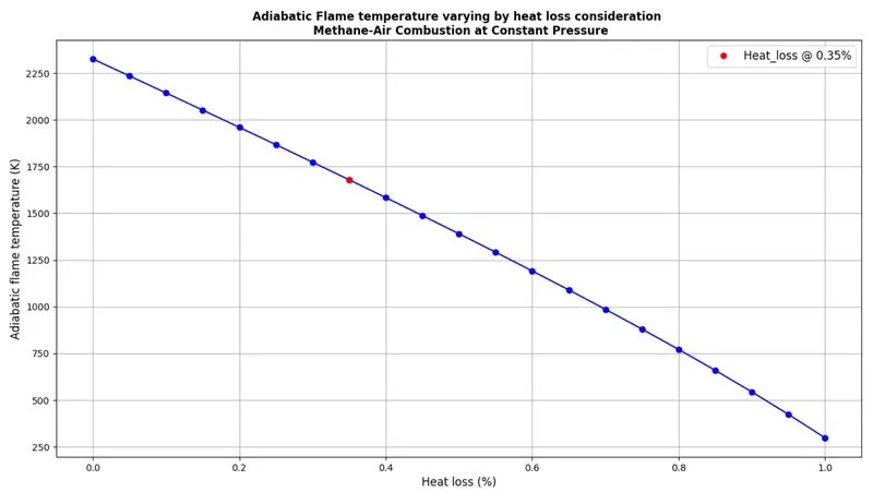
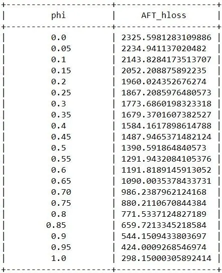
OBSERVATION:
- The plot making sense as the highest temperature recorded at zero heat loss condition and lowest temperature at high heat loss.
- We can observe that at 100 percent heat loss, the AFT recorded is room temperature at which we suppled heat, this shows that the system is not under adiabatic condition.
- And building a system with zero loss is also not possible, because flame loses heat to the environment, or is diluted with an inert material that has to be heated with the heat released in the combustion reaction, the actual temperature reached is less than the ideal adiabatic flame temperature. This is the actual "Flame Temperature."
Adiabatic flame temperature variation with respect to Alkane, Alkene, Alkyne :
We know that fuel is categorized into Alkane, Alkene, Alkyne. In above cases we caluculated the AFT for CH4(Methane) which is an alkane. In this case we will consider all three and plot results. We are considering the combustion taking place at constant pressure with zero loss and stoichometric mixture.
Alkanes, alkenes and alkynes are simple hydrocarbon chains with no functional groups. The simplest organic compounds are the alkanes. Alkanes have only single bonds between carbon atoms and are called saturated hydrocarbons. Alkenes have at least one carbon-carbon double bond. Alkynes have one or more carbon-carbon triple bonds. Alkenes and alkynes are called as unsaturated hydrocarbons. Alkanes have the general formula of CnH2n+2 where n is the number of carbon atoms. Alkenes have the general formula CnH2n. The general formula for alkynes is CnH2n-2.
We know the generic formula for stoichometric mixture for hydrocarbon is CxHy + a(O2 + 3.76N2) = xCO2 + (y/2)H2O + 3.76aN2.
So,
ETHANE: C2H6 + 3.5(O2 + 3.76N2) = 2CO2 + 3H2O + 13.16N2
ETHENE: C2H4 + 3(O2 + 3.76N2) = 2CO2 + 2H2O + 11.28N2
ETHYNE: C2H2 + 2.5(O2 + 3.76N2) = 2CO2 + H2O + 9.4N2
CODE SNIPPET FOR CASE III:
"""
Caluculating adiabatic flame temperature for Alkane(CnH2n+2), Alkene(CnHn), Alkyne(CnH2n-2)
Considering Fuel and air at Stoichometric mixture
ETHANE: C2H6 + 3.5(O2 + 3.76N2) = 2CO2 + 3H2O + 13.16N2
ETHENE: C2H4 + 3(O2 + 3.76N2) = 2CO2 + 2H2O + 11.28N2
ETHYNE: C2H2 + 2.5(O2 + 3.76N2) = 2CO2 + H2O + 9.4N2
Considering the Combustion happening at Constant pressure without heat loss.
"""

import matplotlib.pyplot as plt
import math
import numpy as np
import cantera as ct

"""
We know AFT is caluculated by subracting the enthaplies of products with reactants
"""
#Universal Gas Constant
R = 8.314 #J/mol-K
#Considering the stoichometric combustion
phi = 1
#Function to return the values of enthalpies in joule/mol for each species:
def h(T,co_effs):
	k = co_effs
	return (k[0] + k[1]*T/2 + k[2]*pow(T,2)/3 + k[3]*pow(T,3)/4 + k[4]*pow(T,4)/5 + k[5]/T)*R*T

#coeffiecnts at adiabatic falme temperatura (T<=1000)
ch4_coeffs_l  = [5.14987613E+00, -1.36709788E-02, 4.91800599E-05, -4.84743026E-08, 1.66693956E-11, -1.02466476E+04,-4.64130376E+00]
c2h2_coeffs_l = [8.08681094E-01, 2.33615629E-02, -3.55171815E-05, 2.80152437E-08, -8.50072974E-12, 2.64289807E+04, 1.39397051E+01]
c2h4_coeffs_l = [3.95920148E+00, -7.57052247E-03, 5.70990292E-05, -6.91588753E-08, 2.69884373E-11, 5.08977593E+03, 4.09733096E+00]
c2h6_coeffs_l = [4.29142492E+00, -5.50154270E-03, 5.99438288E-05, -7.08466285E-08, 2.68685771E-11, -1.15222055E+04, 2.66682316E+00]
c3h8_coeffs_l = [0.93355381E+00, 0.26424579E-01, 0.61059727E-05, -0.21977499E-07, 0.95149253E-11, -0.13958520E+05, 0.19201691E+02]
o2_coeffs_l   = [3.78245636E+00, -2.99673416E-03, 9.84730201E-06, -9.68129509E-09, 3.24372837E-12, -1.06394356E+03, 3.65767573E+00]
n2_coeffs_l   = [0.03298677E+02, 0.14082404E-02, -0.03963222E-04, 0.05641515E-07, -0.02444854E-10, -0.10208999E+04, 0.03950372E+02]


#coeffiecnts at adiabatic falme temperatura (T>1000)
co2_coeffs_h = [3.85746029E+00, 4.41437026E-03, -2.21481404E-06, 5.23490188E-10, -4.72084164E-14, -4.87591660E+04, 2.27163806E+00]
co_coeffs_h  = [2.71518561E+00, 2.06252743E-03, -9.98825771E-07, 2.30053008E-10, -2.03647716E-14, -1.41518724E+04, 7.81868772E+00]
h2o_coeffs_h = [3.03399249E+00, 2.17691804E-03, -1.64072518E-07, -9.70419870E-11, 1.68200992E-14, -3.00042971E+04, 4.96677010E+00]
h2_coeffs_h  = [3.33727920E+00, -4.94024731E-05, 4.99456778E-07, -1.79566394E-10, 2.00255376E-14, -9.50158922E+02,-3.20502331E+00]
o2_coeffs_h  = [3.78245636E+00, -2.99673416E-03, 9.84730201E-06, -9.68129509E-09, 3.24372837E-12, -1.06394356E+03, 3.65767573E+00]
n2_coeffs_h  = [0.02926640E+02, 0.14879768E-02, -0.05684760E-05, 0.10097038E-09, -0.06753351E-13, -0.09227977E+04, 0.05980528E+02]

#Function to return the values of enthalpies at given temperature at Constant volume combustion:

def f(T,ntype):


	Tstp = 298.15  #k

	h_ch4_r  = h(Tstp,ch4_coeffs_l)
	h_c2h2_r = h(Tstp, c2h2_coeffs_l)
	h_c2h4_r = h(Tstp, c2h4_coeffs_l)
	h_c2h6_r = h(Tstp, c2h6_coeffs_l)
	h_c3h8_r = h(Tstp, c3h8_coeffs_l)
	h_o2_r   = h(Tstp,o2_coeffs_l)
	h_n2_r   = h(Tstp,n2_coeffs_l)


	h_co2_p = h(T, co2_coeffs_h)
	h_co_p  = h(T, co_coeffs_h)
	h_h2o_p = h(T, h2o_coeffs_h)
	h_h2_p  = h(T, h2_coeffs_h)
	h_o2_p  = h(T, o2_coeffs_h)
	h_n2_p  = h(T, n2_coeffs_h)

	if ntype == 1:           #Alkane is Ethane : CnH2n+2
		x = 2
		y = 6
		fuel = h_c2h6_r
	elif ntype == 2:         #Alkene is Ethene : CnH2n
		x = 2
		y = 4
		fuel = h_c2h4_r
	elif ntype == 3:         #Alkyne is Ethyne : CnH2n-2
		x = 2
		y = 2
		fuel = h_c2h2_r


	H_reactants = fuel + (x + y/4)*	h_o2_r + 3.76*(x + y/4)*h_n2_r
	H_products = x*h_co2_p + (y/2)*h_h2o_p + 3.76*(x + y/4)*h_n2_p

	return(H_reactants - H_products)

#defining a derivative of the above function, Considering forward differencing method:  (f(x+dx)-f(x))/dx):
def fprime(T, ntype):
	return (f(T+1e-6, ntype)-f(T, ntype))/1e-6

ntype = (1,2,3)

AFT = []


for i in range(len(ntype)):
	T_guess = 1500
	alpha = 0.5
	tol = 1e-3
	ct = 1
	while(abs(f(T_guess, ntype[i])) >= tol):
		T_guess = T_guess-((f(T_guess, ntype[i])/fprime(T_guess, ntype[i])))*alpha
		ct = ct+1
	AFT.append(T_guess)


print(ct)
print(AFT)
#plotting the bar graph for the comparision:
x = ['Ethane ($C_2H_6$)', 'Ethene ($C_2H_4$)', 'Ethane ($C_2H_2$)']
y = AFT
plt.bar(x, y, fc = 'lightgray', ec = 'black', width = 0.4)
for i in range (len(ntype)):
	plt.text(i,y[i], round(y[i]), ha = 'center', va = 'bottom')
plt.ylim([2000,3000])
plt.ylabel('Adiabatic Flame Temperature (K)', fontsize = 12)
plt.title('Adiabatic Flame temperature based on type of HydroCarbon', fontsize =13, fontweight ='bold')
plt.show()
Procedure:
- As mentioned in the theory, we copy the values for the co-efficients for the reactants at low temperature and products with high temperature which makes sense.
- We have to define a function for enthalpy(h) for each species with these coefficients and temperature.
- Next we will define a function for caluculating the enthalpy (H) for all reactants(at STP which is known) and products(at AFT which is unknown) by using the above function and at the end equating the difference with zero.
- But we need to find the AFT for ethane, ethene, ethyne. So we define a IF function as n type= [1,2,3].
- By using n values and defining a derivative for the above function using forward differencing method.
- Using newton raphson method, we will iterate to find the value for Adiabatic flame temperature by varying the phi values using a for loop.
- After that using Cantera, we will using the GRI MECH30.xml file to find the solution.
- By using the 'HP' function we will define the temperature, pressure and mole fractions of each reactant in a dictionary, printing the values of AFT by varying the ntype values usnig for loop.
- PLotting the bar chart of AFT caluculated from python.
RESULTS:
OBSERVATION:
- From the plot, we can understand that increase in the value of hydogen results in low AFT temperature because of increase in water components in the products which utilizes the heat. The increase in the Carbon bond strength increases the AFT.
Adiabatic flame temperature variation with respect to a number of Carbon atom chains :
From last case we get to know that increase in carbon strength, so in this case we will capture the resluts by increasing the carbon atoms.
Methane: CH4 + 2(O2 + 3.76N2) = CO2 + 2H2O + 7.52N2
Ethane : C2H6 + 3.5(O2 + 3.76N2) = 2CO2 + 3H2O + 13.16N2
Propane: C3H8 +5(O2 + 3.76N2) = 3CO2 + 4H2O + 18.8N2
CODE SNIPPET FOR CASE IV:
"""
Caluculating adiabatic flame temperature for Alkane(CnH2n+2), Alkene(CnHn), Alkyne(CnH2n-2)
Considering Fuel and air at Stoichometric mixture
Methane: CH4 + 2(O2 + 3.76N2)  = CO2 + 2H2O + 7.52N2
Ethane : C2H6 + 3.5(O2 + 3.76N2) = 2CO2 + 3H2O + 13.16N2
Propane: C3H8 +5(O2 + 3.76N2) = 3CO2 + 4H2O + 18.8N2
Considering the Combustion happening at Constant pressure without heat loss.
"""

import matplotlib.pyplot as plt
import math
import numpy as np

"""
We know AFT is caluculated by subracting the enthaplies of products with reactants
"""

#Universal Gas Constant
R = 8.314 #J/mol-K
#Considering the stoichometric combustion
phi = 1
#Function to return the values of enthalpies in joule/mol for each species:
def h(T,co_effs):
	k = co_effs


	return (k[0] + k[1]*T/2 + k[2]*pow(T,2)/3 + k[3]*pow(T,3)/4 + k[4]*pow(T,4)/5 + k[5]/T)*R*T

#coeffiecnts at adiabatic falme temperatura (T<=1000)
ch4_coeffs_l  = [5.14987613E+00, -1.36709788E-02, 4.91800599E-05, -4.84743026E-08, 1.66693956E-11, -1.02466476E+04,-4.64130376E+00]
c2h6_coeffs_l = [4.29142492E+00, -5.50154270E-03, 5.99438288E-05, -7.08466285E-08, 2.68685771E-11, -1.15222055E+04, 2.66682316E+00]
c3h8_coeffs_l = [0.93355381E+00, 0.26424579E-01, 0.61059727E-05, -0.21977499E-07, 0.95149253E-11, -0.13958520E+05, 0.19201691E+02 ]
o2_coeffs_l   = [3.78245636E+00, -2.99673416E-03, 9.84730201E-06, -9.68129509E-09, 3.24372837E-12, -1.06394356E+03, 3.65767573E+00]
n2_coeffs_l   = [0.03298677E+02, 0.14082404E-02, -0.03963222E-04, 0.05641515E-07, -0.02444854E-10, -0.10208999E+04, 0.03950372E+02]


#coeffiecnts at adiabatic falme temperatura (T>1000)
co2_coeffs_h = [3.85746029E+00, 4.41437026E-03, -2.21481404E-06, 5.23490188E-10, -4.72084164E-14, -4.87591660E+04, 2.27163806E+00]
co_coeffs_h  = [2.71518561E+00, 2.06252743E-03, -9.98825771E-07, 2.30053008E-10, -2.03647716E-14, -1.41518724E+04, 7.81868772E+00]
h2o_coeffs_h = [3.03399249E+00, 2.17691804E-03, -1.64072518E-07, -9.70419870E-11, 1.68200992E-14, -3.00042971E+04, 4.96677010E+00]
h2_coeffs_h  = [3.33727920E+00, -4.94024731E-05, 4.99456778E-07, -1.79566394E-10, 2.00255376E-14, -9.50158922E+02,-3.20502331E+00]
o2_coeffs_h  = [3.78245636E+00, -2.99673416E-03, 9.84730201E-06, -9.68129509E-09, 3.24372837E-12, -1.06394356E+03, 3.65767573E+00]
n2_coeffs_h  = [0.02926640E+02, 0.14879768E-02, -0.05684760E-05, 0.10097038E-09, -0.06753351E-13, -0.09227977E+04, 0.05980528E+02]

#Function to return the values of enthalpies at given temperature at Constant volume combustion:
def f(T,n):


	Tstp = 298.15  #k

	h_ch4_r  = h(Tstp,ch4_coeffs_l)
	h_c2h6_r = h(Tstp, c2h6_coeffs_l)
	h_c3h8_r = h(Tstp, c3h8_coeffs_l)
	h_o2_r   = h(Tstp,o2_coeffs_l)
	h_n2_r   = h(Tstp,n2_coeffs_l)


	h_co2_p = h(T, co2_coeffs_h)
	h_co_p  = h(T, co_coeffs_h)
	h_h2o_p = h(T, h2o_coeffs_h)
	h_h2_p  = h(T, h2_coeffs_h)
	h_o2_p  = h(T, o2_coeffs_h)
	h_n2_p  = h(T, n2_coeffs_h)


	if n == 1:           #Methane
		x = 1
		y = 4
		fuel = h_ch4_r
	elif n == 2:         #Ethane
		x = 2
		y = 6
		fuel = h_c2h6_r
	elif n == 3:        #Propane
		x = 3
		y = 8
		fuel = h_c3h8_r

	#CxHy+a(O2+3.56N2)
	H_reactants = fuel + (x + y/4)*	h_o2_r + 3.76*(x + y/4)*h_n2_r
	H_products = x*h_co2_p + (y/2)*h_h2o_p + 3.76*(x + y/4)*h_n2_p


	return(H_reactants - H_products)

#defining a derivative of the above function, Considering forward differencing method:  (f(x+dx)-f(x))/dx):
def fprime(T, n):
	return (f(T+1e-6, n)-f(T, n))/1e-6

n = [1,2,3]

AFT = []


for i in range(len(n)):
	T_guess = 1500
	alpha = 0.5
	tol = 1e-3
	ct = 1
	while(abs(f(T_guess, n[i])) >= tol):
		T_guess = T_guess-((f(T_guess, n[i])/fprime(T_guess, n[i])))*alpha
		ct = ct+1
	AFT.append(T_guess)


print(ct)
print(AFT)
#plotting the bar graph for the comparision:
x = ['Methane ($CH_4$)', 'Ethane ($C_2H_6$)', 'Propane ($C_3H_8$)']
y = AFT
plt.bar(x, y, fc = 'lightgray', ec = 'black', width= 0.5)
for i in range (len(x)):
	plt.text(i,y[i], round(y[i]), ha = 'center', va = 'bottom')

plt.ylim([2200,2450])
plt.ylabel('Adiabatic Flame Temperature (K)', fontsize = 12)
plt.title('Adiabatic Flame temperature based on number of Carbon atoms', fontsize =13, fontweight ='bold')
plt.show()
RESULTS:
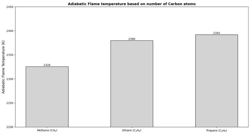
OBSERVATION:
- We can observe that increase in carbon atoms in reactants which forms more CO2 in prodcuts increases the AFT.
- But for Ethane and propane, we can observe less difference, this is because even though increase in CO2 in products, there is an parallel increase in the water components which utilises the heat.
CONCLUSION:
From all the above studies, I conclude that to get high adiabatic flame temperature, we have to consider following :
- The fuel and air has to be at stoichometric conditions. Lean mixture leads to less combustion and rich mixture leads to negative heat.
- The heat loss should be minimal.
- Decraese in hydrogen atoms in fuel will gives high AFT.
- Increase in Carbon atoms leads to high AFT.