Week 8 - BlockMesh Drill down challenge
BlockMesh Drill down challenge
Objective: To simulate an incompressible-laminar-viscous flow through the backward facing step geometry using transient simulation and the solver is choosen based on the physics of the flow.
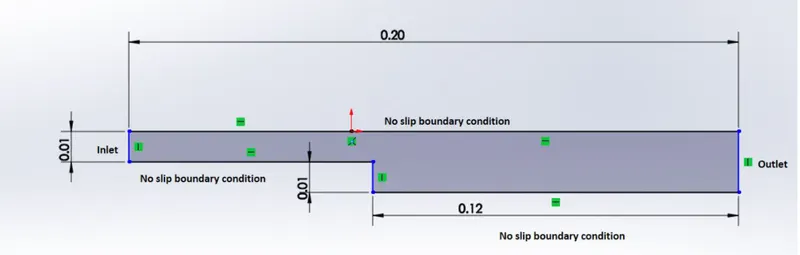
The case involved here is incompressible laminar viscous flow through two dimensional blockmesh. Initially the flow is considered as laminar flowand will be solved on a uniform mesh using the icoFoam solver for laminar and incompressible flow. ICOFOAM is a transient solver used to solve the incompressible laminar Navier stokes equation using PISO algarithm as it requires initial and boundary conditions.
In practice to simulate any project every CFD engineers must follow three phases:
1. Pre Processing
2. Processing
3. Post Processing.
The Pre Processing includes :
Geometry creation or Import: Any case is setup by editing or modifying the case files by using gedit tool available in open foam. Editing files is possible in OpenFOAM because the I/O uses a dictionary format with keywords that convey sufficient meaning to be understood by the users.
Any case simulated in Openfoam consists of mesh, initail conditions and other parameters. After understanding the type of problem we are dealing with, we have to select case realted with existing cases in the tutorials folder. After that we have to copy that case file into run folder as open foam doesnot aloow us to modify the tutorials.
In our case, we have selected the case is solving using ICOFOAM solver aand we are copying the case related to the solver from tutorials folder to run folder by using following commands in termimal.
cd $FOAM_RUN
cp -r $FOAM_TUTORIALS/incompressible/icoFoam/cavity/cavity .
cd cavity
After that we have to edit the blockmeshdict file present inside the system folder of the case file.
To avail blockMeshDict file, cd system
gedit blockMeshDict
Before editing the case, we have to prepare the geometry of the case as follows:

GEOMETRY PREPARATION:
As per the above diagram, we have to note them in node wise and edit the case file accordingly.
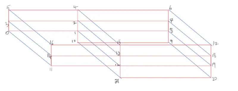
BLOCKMESHDICT FILE:
/*--------------------------------*- C++ -*----------------------------------*\
  =========                 |
  \\      /  F ield         | OpenFOAM: The Open Source CFD Toolbox
   \\    /   O peration     | Website:  https://openfoam.org
    \\  /    A nd           | Version:  8
     \\/     M anipulation  |
\*---------------------------------------------------------------------------*/
FoamFile
{
    version     2.0;
    format      ascii;
    class       dictionary;
    object      blockMeshDict;
}
// * * * * * * * * * * * * * * * * * * * * * * * * * * * * * * * * * * * * * //

convertToMeters 0.01;  // As the problem mentioned in meters and here we are taking in centimeters, we are using correction factor

vertices
(
    (0 0 0)        //[0]
    (8 0 0)        //[1]
    (8 0.5 0)      //[2]
    (0 0.5 0)      //[3]
    (8 1 0)        //[4]
    (0 1 0)        //[5]
    (20 1 0)       //[6]
    (20 0.5 0)     //[7]
    (20 0 0)       //[8]
    (20 -1 0)       //[9]
    (8 -1 0)       //[10]
    (0 0 0.1)      //[11]
    (8 0 0.1)      //[12]
    (8 0.5 0.1)    //[13]
    (0 0.5 0.1)    //[14]
    (8 1 0.1)      //[15]
    (0 1 0.1)      //[16]
    (20 1 0.1)     //[17]
    (20 0.5 0.1)   //[18]
    (20 0 0.1)     //[19]
    (20 -1 0.1)    //[20]
    (8 -1 0.1)     //[21]
);

blocks
(
    hex (0 1 2 3 11 12 13 14) (80 5 1) simpleGrading (1 1 1)
    hex (3 2 4 5 14 13 15 16) (80 5 1) simpleGrading (1 1 1)
    hex (2 7 6 4 13 18 17 15) (120 5 1) simpleGrading (1 1 1)
    hex (1 8 7 2 12 19 18 13) (120 5 1) simpleGrading (1 1 1)
    hex (10 9 8 1 21 20 19 12) (120 10 1) simpleGrading (1 1 1)
);

edges
(
);

boundary
(
    inlet
    {
        type patch;
        faces
        (
            (0 11 14 3)
            (3 14 16 5)
        );
    }
    outlet
    {
        type wall;
        faces
        (
            (7 6 17 18)
            (8 7 18 19)
            (9 8 19 20)
        );
    }

    frontAndBack
    {
        type empty;
        faces
        (
            (0 3 2 1)
            (3 5 4 2)
            (2 4 6 7)
            (1 2 7 8)
            (10 1 8 9)
            (11 12 13 14)
            (13 15 16 14)
            (18 17 15 13)
            (19 18 13 12)
            (20 19 12 21)
        );
    }

    NoslipWalls
    {
        type wall;
        faces
        (
            (5 16 15 4)
            (4 15 17 6)
            (0 1 12 11)
            (10 9 20 21)
            (10 21 12 1)
        );
    }
);

mergePatchPairs
(
);

// ************************************************************************* //
MESH GENERATION: The mesh is generated by running blockMesh on this blockMeshDict file. From within the case directory, this is done, simply by typing in the terminal.The running status of blockMesh is reported in the terminal window. Any mistakes in the blockMeshDict file are picked up by blockMesh and the resulting error message directs the user to the line in the file where the problem occurred. There should be no error messages at this stage.
BOUNDARY AND INTIAL CONDITIONS:
After creating the mesh, we have to set up the boundary and initial conditions. This can be done by editing the 0 file present inside the case file(cavity) we can get this by typing the following in terminal window:
cd cavity
cd cavity
cd 0
By listing the 0 file, we will observe two files as like p,U, these are initial condition files for pressure and velocity which has to be edited according to the case as follows:
INITIAL CONDITION FOR VELOCITY:
/*--------------------------------*- C++ -*----------------------------------*\
  =========                 |
  \\      /  F ield         | OpenFOAM: The Open Source CFD Toolbox
   \\    /   O peration     | Website:  https://openfoam.org
    \\  /    A nd           | Version:  8
     \\/     M anipulation  |
\*---------------------------------------------------------------------------*/
FoamFile
{
    version     2.0;
    format      ascii;
    class       volVectorField;
    object      U;
}
// * * * * * * * * * * * * * * * * * * * * * * * * * * * * * * * * * * * * * //

dimensions      [0 1 -1 0 0 0 0];

internalField   uniform (0 0 0);

boundaryField
{
   inlet
    {
        type            fixedValue;
        value           uniform (1 0 0);
    }

    outlet
    {
        type            zeroGradient;

    }


    frontAndBack
    {
        type            empty;
    }

    NoslipWalls
    {
        type            noSlip;
    }
}

// ************************************************************************* //
INITIAL CONDITION FOR PRESSURE:
/*--------------------------------*- C++ -*----------------------------------*\
  =========                 |
  \\      /  F ield         | OpenFOAM: The Open Source CFD Toolbox
   \\    /   O peration     | Website:  https://openfoam.org
    \\  /    A nd           | Version:  8
     \\/     M anipulation  |
\*---------------------------------------------------------------------------*/
FoamFile
{
    version     2.0;
    format      ascii;
    class       volScalarField;
    object      p;
}
// * * * * * * * * * * * * * * * * * * * * * * * * * * * * * * * * * * * * * //

dimensions      [0 2 -2 0 0 0 0];

internalField   uniform 0;

boundaryField
{
   inlet
    {
        type            zeroGradient;
    }

    outlet
    {
        type            fixedValue;
        value           uniform 0;
    }


    frontAndBack
    {
        type            empty;
    }

    NoslipWalls
    {
        type            zeroGradient;
    }

}

// ************************************************************************* //
NOTE:
Whatever the walls and patches mentioned in blockmeshdict file has to be mentioned in initial conditions such as dimensions, internal field and boundary field. In this case the boundary consits of walls split into three patches named as inlet & outlet, front and back and no slip walls.
CONTROL DICT FILE:
Input data relating to the control of time and reading and writing of the solution data are read in from the controlDict dictionary. The user should view this file; as a case control file, it is located in the system directory.
cd cavity/cavity/
cd system/
gedit controlDict
/*--------------------------------*- C++ -*----------------------------------*\
  =========                 |
  \\      /  F ield         | OpenFOAM: The Open Source CFD Toolbox
   \\    /   O peration     | Website:  https://openfoam.org
    \\  /    A nd           | Version:  8
     \\/     M anipulation  |
\*---------------------------------------------------------------------------*/
FoamFile
{
    version     2.0;
    format      ascii;
    class       dictionary;
    location    "system";
    object      controlDict;
}
// * * * * * * * * * * * * * * * * * * * * * * * * * * * * * * * * * * * * * //

application     icoFoam;

startFrom       startTime;

startTime       0;

stopAt          endTime;

endTime         0.5;

deltaT          0.0001;

writeControl    timeStep;

writeInterval   20;

purgeWrite      0;

writeFormat     ascii;

writePrecision  6;

writeCompression off;

timeFormat      general;

timePrecision   6;

runTimeModifiable true;


// ************************************************************************* //
Open foam provides us the flexibility to choose the start and stop time of the simulation. Here the start time is 0 and the end time is 0.5. Now we have to select the value for delta t as it plays major role in setting up the courant number which needs to be less than 1 to get convergence and numerical stability.
As we know
As per the given data, we know that the length along x-axis is 0.2m and y- axis is 0.02 and the mesh specifications are 200 and 20 respectively.
so dx = 0.2/200 = 0.001 s.
So the delta t value is taken as 0.0001 to meet the courant number criteria.Let us decide that we wish to write our results at times 0.1, 0.2,…, 0.5 s. With a time step of 0.005 s, we therefore need to output results at every 20th time time step and so we set writeInterval to 20.
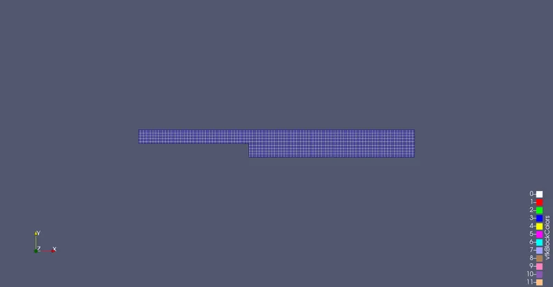
After completing all the above steps, we have to view the mesh by using paraFoam command in the terminal before processing the case. This is because to know the mesh created correctly or not. the output for the case is
PROCESSING THE CASE:
OpenFOAM applications can be run either in the foreground or background. On this occasion, we will run icoFoam in the foreground. The icoFoam solver is executed either by entering the case directory and typing at the command prompt, or with the optional -case argument giving the case directory
If everything went right means we will get the convergence or esle an error message will appear on terminal showing where the error has happenned. If we get the solution, we can view the result in the post processing step using the command in terminal
cd cavity/
paraFoam
We will see the results by using an inbuilt software named as paraview.
Post-processing
As soon as results are written to time directories, they can be viewed using paraFoam. Return to the paraFoam window and select the Properties panel for the cavity.OpenFOAM case module. If the correct window panels for the case module do not seem to be present at any time, please ensure that: cavity.OpenFOAM is highlighted in blue eye button alongside it is switched on to show the graphics are enabled.
OUTPUTS:
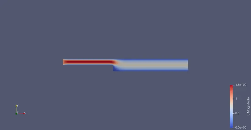
VELOCITY VARIATION NEAR THE STEP:
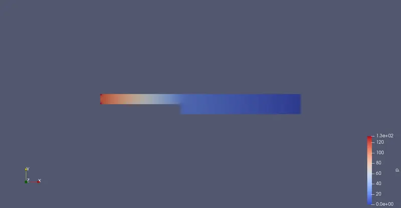
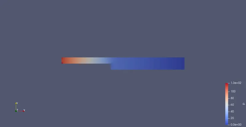
PRESSURE VARIATION:
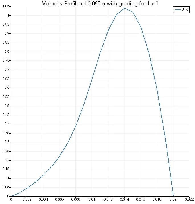
VELOCITY PROFILE AT 0.085 M NEAR THE STEP:
CASE-II
Simulate the flow with grading factor of 0.2:
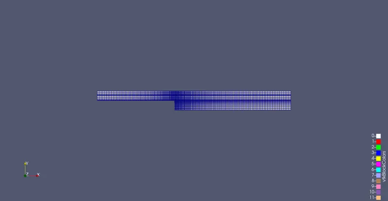
Everything will be similat to the case-I but the only difference is that editing the blockMeshDict file to modify the grading factor. Grading factor is essential for mesh refining and is explained as the expansion ratio enables the mesh to be graded, or refined, in specified directions. The ratio is that of the width of the last cell (L) along one edge of a block to the width of the first cell (F) along that edge. If the mesh is uniform along all directions then it is called as simple grading. But in some caes the mesh has to streched along onr particular direction, then by using grading factor we will define the mesh size.
Grading factor, f = size of last cell(L) / size of First cell (F).
CODE FOR BLOCKMESHDICT FILE:
hex (0 1 2 3 11 12 13 14) (80 5 1) simpleGrading (0.2 5 1)
    hex (3 2 4 5 14 13 15 16) (80 5 1) simpleGrading (0.2 5 1)
    hex (2 7 6 4 13 18 17 15) (120 5 1) simpleGrading (5 5 1)
    hex (1 8 7 2 12 19 18 13) (120 5 1) simpleGrading (5 5 1)
    hex (10 9 8 1 21 20 19 12) (120 10 1) simpleGrading (5 0.2 1)
RESULTS:
MESH GENERATION:
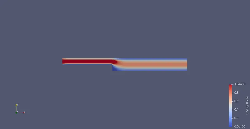
VELOCITY VARIATION PLOT:
PRESSURE VARIATION PLOT:
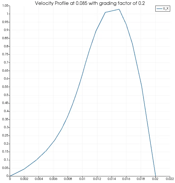
VELOCITY PROFILE AT 0.085 M NEAR THE STEP:
COMPARISION TABLE:
| PROPERTIES | GRADING FACTOR = 1 | GRADING FACTOR = 0.2 |
| VELOCITY | 0.6516 | 0.6350 |
| PRESSURE | 16.9009 | 16.7824 |
| SIMULATION TIME | 53.77S | 52.05 |
NOTE: the velocity and pressure values are taken at 0.085m and at center 0.0005.
The main difference observed from the velocity profile plots are that eventhough the plot with grading factor of 1 is smooth compared to 0.2, the later plot provides exact information which i feels. And by looking at the values of pressure and velocity from table also shows that the mesh with finer are low. Morever the simulation time also less comparatively with grading factor of 1.
CONCLUSION:
Grading/growth factors gives us the freedom of generating refine mesh along particular direction which helps in most cases to concentrate at particular place. If the mesh is finer we will get the information at that point will be almost exact with less simulation time.