Week 9 - FVM Literature Review

FINITE VOLUME METHOD LITERATURE REVIEW

As we know CFD is most reliable way to deal with several problems, mainly in the development of mathematical models to describe the process and the application of appropriate numerical method to solve the proposed model. The main objective in doing such practices is to obey the conservation laws at every point in the control volume, which means the mass, energy and momentum should be conserved with out generation or obsrervation of internal terms in the control volume. There are so many techniques available to solve these equations, some important methodolgies are : Finite Difference Method (FDM), Finte Volume Method (FVM) and Finite element Method (FEM).

The FVM is currently the most common method used to solve fluid flow problems. This popularity is directly related to its conservative nature, since in flow simulations it is extremely important to satisfy the conservation laws at all levels, avoiding generation/consumption of mass, energy, or momentum due to artificial terms inside the control volume, independent of the mesh size. The same is not guaranteed in finite difference and finite element methods.

FINITE VOLUME METHOD:

"Finite volume" means a very small volume. Finite volume method is a mathematical technique used to transform the partial differtial equations into the form of algebaric equations which is to be conserved. The process involves in FVM is to convert the volume integrals of the partial differential equations into the surface integarls using divergence theorem. Then these terms are converted to fluxes at the surface of the each finite volume. The notation of the fluxes here are to meaningfull because these has to be conserved which means the flux entering the volume should be equal to the flux exiting the volume. This type of conserving the quantities is not possible in FDM & FEM which is caluculated using approximations from nodal and local data. But when it comes to FVM, the solution to be exact for the average value of the solution over some volume, and uses this data to construct approximations of the solution within cells.

Steps involved in FVM:

a) Defining the partial differential equations of governing equations into integral form.

b) Converting the volume integrals into surface integrals using Gauss divergence theorem.

c) Writing these surface integrals into flux terms which is to algebraic form.

The major differences between FDM & FVM are as below:

1) The properties of the quantities are caluculated from nodal data by using approximations untill the solution is conserved in FDM where as in FVM, the quatities are caluculated for a small control volume and then integrating for whole control volume.

2) FDM is very usefull for orthogonally cartesian co-ordinates, but it can be used over irregular arbitary shapes in FVM.

3) The solution may not be necessarirly conserved in FDM, when it comes to FVM the solution will be conserved at every volume.

4) It is very difficult to use for handling material discontinues in FDM.

5) The functions that approximate the solution when using the finite-volume method cannot be easily made of higher order. It is possible in finite difference method by increasing the element order.

NEED OF INTERPOLATION SCHEMES IN FVM:

The approximation of surface and volume integrals may require values of the variable at locations other than the computational nodes of the CV. Values at these locations are obtained using interpolation formulae.

Various schemes of interpolation methods in FVM:

a) UpWind Interpolation. (UDS)

b) Linear Interpolation. (CDS)

c) Quardratic UpWind Interpolation for convective kinematics. (QUICK)

d) Hybrid Interpolation.

e) Total variation Diminishing.(TVD)

f) Essentially Non Oscillation Interpolation (ENO)

UpWind Interpolation:

UpWind interpolation is used for approximating the value of a variable f at east face of control volume which is given by

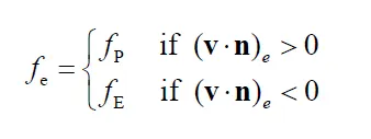
• Upwind interpolation simply UDS is equivalent to using a backward or forward differencing method approximation which is dependant on flow direction. As mention in the above statement if the velocity component at face point e is greater than at P then we will use forward differencing technique.
• UDS is an first ordre accuarte approximation in which we will ignore O(dx).
• It is very popular because of minimising of damping properties as it is numerically diffusive with a coefficient of numerical diffusion y = (rho.Ue) dx / 2.
• UDS is the only approximation which satisfy boundedness even if the velocity has peak variations also.

Linear Interpolation:

We can approximate the value of the variable at CV face centre by linear interpolation of the values at two nearest computational nodes. Thus, at location ‘e’ on a Cartesian grid, the variable value is approximated by

where `lamda` = waiting finction..

• It is very equivalent to central differencing method with first order accurate, So that this scheme also called as central differencing scheme (CDS).
• This technique is simplest and most widely used interpolation.
• It may produce oscillatory solutions as the grid spacing considered is more.
• Approximation of gradients has second order accuracy on uniform grids, whereas formally of first order accuracy on non- uniform grids.

Quardratic UpWind Interpolation for convective kinematics :

A quadratic upwind interpolation (QUICK) scheme can be derived using polynomial fitting. The QUICK interpolation on a uniform Cartesian grid is given by

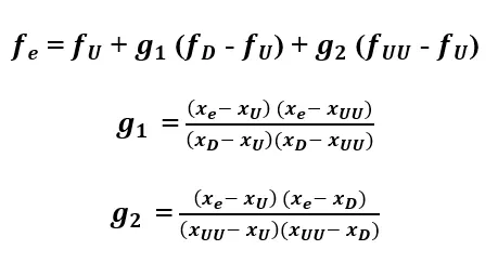
where D, U and UU denote the downstream, the first upstream and the second upstream node respectively (E, P, and W or P, E and EE depending on the flow direction.

• This method considers second order accurate terms and ignores third order terms, Such it is of third order accurate method.
• This method superior in terms of both accuracy and reducing damping properties compared to UDS & CDS.

Hybrid Interpolation:

It is a blend of both CDS and UDS interpolation methods depends on local peclet number which is given by

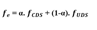
if the local peclet number is near to one, then we will go with CDS method or esle both methods are used to increase accuracy and to reduce damping properties.

Total variation Diminishing:

In Numerical methods, total variation diminishing (TVD) is a property of certain discretization schemes used to solve hyperbolic partial differential equations which is given by

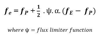
FLUX LIMITERS IN FINITE VOLUME METHOD:

• The flux limiters are mainly used in higher order schemes to reduce oscillations that would otherwise occur with high order spatial discretization schemes due to shocks, discontinuities or sharp changes in the solution domain.
• These are also called as slope limiters because they both have the same mathematical form, and both have the effect of limiting the solution gradient near shocks or discontinuities.
• Use of flux limiters, together with an appropriate high resolution scheme, make the solutions total variation diminishing (TVD).
• By looking at the tvd form, we will understand that if the flux limter is equal to zero the we will go with low resolution schemes. Similarly if it is equal to one, then we will go with high resolution scheme.
• The main objective of impelementing of flux limiters is that to control the spatila derivatives to realistic values.

By taking an example of 1D heat conduction equation:

Let consider a control volume as shown below

where, P is the centre of control volume and W & E is the left & right neighbouring contro volumes. And the w and e are face points.

As we know the general 1D heat conduction equation is of

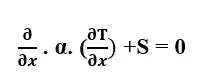
Where,

S is source term

α is a function of temperature.

Now considering a small volume from control volume P and integrating it.

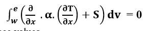
As the limits w and e are face values.

As we know the dv is equal to A. dx.

Then the above equation is written as

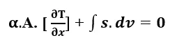
By using taylor’s series approximation, the above equation will becomes to

In the above equation, if the source term is the function of temperature then by doing linearization to it becomes

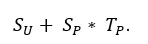
The value of Tp will be calculated by using interpolation methods.

Now coming to the heat conduction equation,

By looking at the above equation, its very clear that outward flux - inward flux + source terms are equal to zero in which the quantities are conserved. Such that in FVM the quantities will be conserverd at every volume entering and at the exiting.