Week 7 - Simulation of a 1D Super-sonic nozzle flow simulation using Macormack Method

Objective:

The main objective of this challenge is to implement all the CFD techniques which we have learned so far. In some cases, more than one CFD technique will be used to solve the same flow problem. This is done to give you some comparison of the strengths and weakness of one technique versus another and a feeling for the relative difficulty of setting up one technique on the computer compared to another.

The solution is computed by MacCormack technique, which is an explicit finite difference scheme that is very popular in CFD. The MacCormack method is multi-level, meaning that there is a multistep process to reach the solution. These steps are traditionally called predictor and corrector, where an averaging can then be performed. The averaging at each time step is what allows for the higher accuracy while using a relatively simple finite difference scheme.

NOTE: A step-by-step procedure of the MacCormack method can be found in Anderson.

INITIAL SETUP OF THE PROBLEM:

We are considering the steady, isentropic flow through a convergent and divergent nozzle as below. The flow properties are defined at inlet and outlet as mentioned in the figure as the nozzle is connected to a reservoir where area tends to infinity.

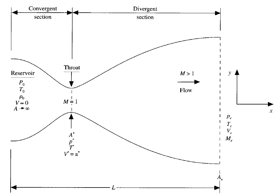
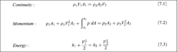
Even though the flow is in both X and Y directions, we are assuming the flow is Quasi One-Dimensional flow. As we already know the set of governing equations for quasi 1D flow as follows:

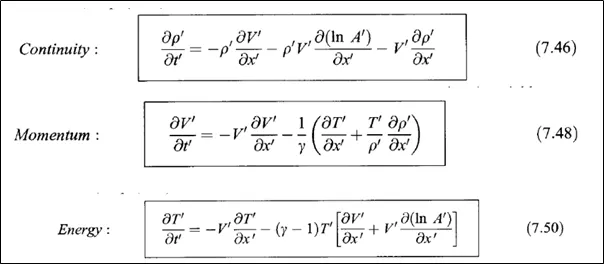
After introducing Non-Dimensional variables, the following set of equations will get for Non conservative form:

For Conservative form:

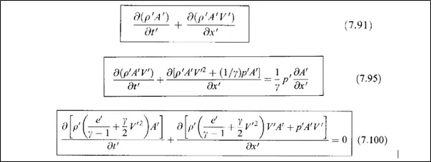
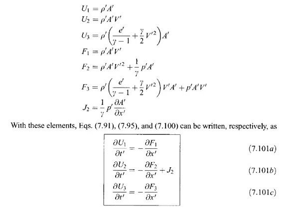
The equations for Quasi 1D flow can be expressed in generic form. Let us define the elements of the solutions vector as U, the flux vector as F and the Source term as J as follows:

Octave Function program for Non-Conservative form:

function [v,rho,t,m,mach,pr,v_t,rho_t,t_t,m_t,mach_t,pr_t] = Non_conservative_form(L,n,c,nt,throat)
% Initial variables
x = linspace(0,L,n);
dx = x(2)-x(1);

% initial profiles of non dimensional numbers
rho = 1-0.3146*x;                %density
t = 1-0.2314*x;                  %temperature
v = (0.1+1.09*x).*t.^0.5;        %velocity
a = 1+2.2*(x-1.5).^2;            %area
gamma = 1.4;                     %adiabatic index

% Caluculating time step using courant number criteria
for i = 1:n
del_t(i) = c*(dx/(t(i)^0.5+v(i)));
endfor
% Minimum value of delta t will give more accutacy
dt = min(del_t)

%outer time loop
for k = 1:nt
  % saving old values
  rho_old = rho;
  v_old= v;
  t_old = t;
  %predictor method
  for j = 2:n-1
    dvdx = (v(j+1)-v(j))/dx;
    drhodx = (rho(j+1)-rho(j))/dx;
    dtdx = (t(j+1)-t(j))/dx;
    dlogadx = (log(a(j+1))-log(a(j)))/dx;
    
    % continuity equation
    drhodt_p(j) = -rho(j)*dvdx-rho(j)*v(j)*dlogadx-v(j)*drhodx;
    %momentum equation
    dvdt_p(j) = -v(j)*dvdx-(1/gamma)*(dtdx+((t(j)/rho(j))*drhodx));
    %energy equation
    dtdt_p(j) = -v(j)*dtdx-(gamma-1)*t(j)*(dvdx+v(j)*dlogadx);
    
    %updating old values
    rho(j) = rho(j)+drhodt_p(j)*dt;
    v(j) = v(j)+dvdt_p(j)*dt;
    t(j) = t(j)+dtdt_p(j)*dt;
  endfor
  
  %corrector method
  for j = 2:n-1
    dvdx = (v(j)-v(j-1))/dx;
    drhodx = (rho(j)-rho(j-1))/dx;
    dtdx = (t(j)-t(j-1))/dx;
    dlogadx = (log(a(j))-log(a(j-1)))/dx;
    
    % Continuity equation
    drhodt_c(j) = -rho(j)*dvdx-rho(j)*v(j)*dlogadx-v(j)*drhodx;
    % Momentum equation
    dvdt_c(j) = -v(j)*dvdx-(1/gamma)*(dtdx+((t(j)/rho(j))*drhodx));
    %Energy equation
    dtdt_c(j) = -v(j)*dtdx-(gamma-1)*t(j)*(dvdx+v(j)*dlogadx);
     
  endfor
  
  % co mputing the average values
    drhodt  = 0.5*(drhodt_p+drhodt_c);
    dvdt    = 0.5*(dvdt_p+dvdt_c);
    dtdt    = 0.5*(dtdt_p+dtdt_c);
  
  %final solution update
  for i = 2:n-1
    rho(i) = rho_old(i)+drhodt(i)*dt
    v(i)   = v_old(i) +dvdt(i)*dt
    t(i)   = t_old(i)+ dtdt(i)*dt
  endfor
  
  
  % boundary conditions
  rho(1) = 1;
  v(1) = 2*v(2)-v(3);
  t(1) = 1;
  
  %final boundary
  rho(n) = 2*rho(n-1)-rho(n-2);
  v(n) = 2*v(n-1)-v(n-2);
  t(n) = 2*t(n-1)-t(n-2);
  
  % Caluculating mass flow rate
  m = rho.*a.*v;
  
  %caluculating pressure
  pr = rho.*t
  
  % caluculating mach number
  mach = v./(t.^0.5);
  
% Caluculating flow variables at throat
v_t(k) = v(throat);
rho_t(k) = rho(throat);
t_t(k) = t(throat);
m_t(k) = m(throat);
pr_t(k) = pr(throat);
mach_t(k) = mach(throat);


% Plotting mass flow rate by varying time steps
  figure(1)
 if k==50
   plot(x,m,'r', 'linewidth',1.5);
   hold on
 elseif k == 100
   plot(x,m,'b', 'linewidth',1.5);
   hold on
 elseif k == 200
   plot(x,m,'g', 'linewidth',1.5);
   hold on
 elseif k == 500
   plot(x,m,'k', 'linewidth',1.5);
   hold on
 elseif k == 700
   plot(x,m,'c', 'linewidth',1.5);
   hold on
 elseif k == 1400
   plot(x,m,'y', 'linewidth',1.5);
  
 xlabel('Distance through Nozzle along X-Axis');
 ylabel('Non_Dimensional Flow Rate');
 title(sprintf('Comparision of mass flow rate at Different time steps'));
 legend({'50 timesteps','100 timesteps','200 timesteps','500 timesteps','700 timesteps','1400 timesteps'})
 end
endfor
endfunction

Octave Function program for Conservative form:

function [v,rho,t,m,mach,pr,v_t,rho_t,t_t,m_t,mach_t,pr_t] = Conservative_form(L,c,n,nt,throat)
  % Initial variables
  x = linspace(0,L,n);
  dx= x(2)-x(1);
  a= 1+2.2*(x-1.5).^2;
for i = 1:n
  if (x(i)>=0 && x(i)<=0.5)
    rho(i) = 1;
    t(i)   = 1;
  elseif (x(i)>=0.5 && x(i)<=1.5)
    rho(i) = 1-0.366*(x(i)-0.5);
    t(i)   = 1-0.167*(x(i)-0.5);
    elseif(x(i)>=1.5 && x(i)<=3.5)
    rho(i) = 0.634-0.3879*(x(i)-1.5);
    t(i)   = 0.833-0.3507*(x(i)-1.5);
  endif
endfor

 
  % Initial conditions
  v = 0.59./(rho.*a);
  gamma = 1.4;
  
  % Solution vector parameters
  pr = rho.*t;
  u1 = rho.*a;
  u2 = rho.*a.*v;
  u3 = u1.*((t./(gamma-1))+(gamma/2).*(v.^2));
  
  %Caluculating the time step using courant number
  %dt = min (c.*(dx./(t.^0.5)+v));
   dt = 0.0267;
  %outer time loop
  for k = 1:nt
    %saving old values
    u1_old = u1;
    u2_old = u2;
    u3_old = u3;
    
    
    % Pure form of the flux terms
    f1 = u2;
    f2 = (u2.^2./u1)+((gamma-1)/gamma)*(u3-(gamma/2)*(u2.^2./u1));
    f3 = gamma*((u2.*u3)./u1)-(gamma*(gamma-1)/2)*(u2.^3./u1.^2);
    
    % predictor method
    for j = 2:n-1
      df1dx(j) = (f1(j+1)-f1(j))/dx;
      df2dx(j) = (f2(j+1)-f2(j))/dx;
      df3dx(j) = (f3(j+1)-f3(j))/dx;
      dadx(j) = (a(j+1)-a(j))/dx;
      j2(j) = (1/gamma)*rho(j)*t(j)*dadx(j);
      
      % Continuity equation
      du1dt_p(j) = -df1dx(j);
      
      % Momentum equation
      du2dt_p(j) = -df2dx(j)+j2(j);
      
      %energy equation
      du3dt_p(j)= -df3dx(j);
      
      % Solution update
      u1(j) = u1(j) + du1dt_p(j)*dt;
      u2(j) = u2(j) + du2dt_p(j)*dt;
      u3(j) = u3(j) + du3dt_p(j)*dt;
    endfor
 
  % Getting primitive terms from above data
    
    rho = u1./a;
    v = u2./u1;
    t = (gamma-1)*((u3./u1)-(gamma*v.^2./2));
    
    % Pure form of flux terms for corrector step.
    f1 = u2;
    f2 = (u2.^2./u1)+((gamma-1)/gamma)*(u3-(gamma/2)*(u2.^2./u1));
    f3 = gamma*((u2.*u3)./u1)-(gamma*(gamma-1)/2)*(u2.^3./u1.^2);
    
    % corrector step
    for j = 2:n-1
     df1dx(j) = (f1(j)-f1(j-1))/dx;
      df2dx(j) = (f2(j)-f2(j-1))/dx;
      df3dx(j) = (f3(j)-f3(j-1))/dx;
      dadx(j) = (a(j)-a(j-1))/dx;
      j2(j) = (1/gamma)*rho(j)*t(j)*dadx(j);
      
      % Continuity equation
      du1dt_c(j) = -df1dx(j);
      
      % Momentum equation
      du2dt_c(j) = -df2dx(j)+j2(j);
      
      %energy equation
      du3dt_c(j)= -df3dx(j);
      
    endfor
    
     % average derivative
    
    du1dt = 0.5*(du1dt_p+du1dt_c);
    du2dt = 0.5*(du2dt_p+du2dt_c);
    du3dt = 0.5*(du3dt_p + du3dt_c);
    
    % final solution
    for i = 2:n-1
      u1(i) = u1_old(i)+du1dt(i)*dt;
      u2(i) = u2_old(i)+du2dt(i)*dt;
      u3(i) = u3_old(i)+du3dt(i)*dt;
    endfor
    
      % boundary conditions
    % At Inlet
    % Before setting up the boundary conditions, we shuold note that "rho" is fixed and independant value 
     u1(1) = rho(1)*a(1);
     u2(1) = 2*u2(2)-u2(3); %As u2 consists of floatinf value "v", which is caluculated from internal grid points
     v(1)= u2(1)/u1(1);
     u3(1) = u1(1)*((t(1)/(gamma-1))+(gamma/2)*v(1)^2);
     
     % At Outlet 
     % The flow properties at outlet will get from internal grid points at "n"
     u1(n) = 2*u1(n-1)-u1(n-2);
     u2(n) = 2*u2(n-1)-u2(n-2);
     u3(n) = 2*u3(n-1)-u3(n-2);
     
     % Caluculating Primitive terms
     rho = u1./a;
     v = u2./u1;
     t = (gamma-1)*((u3./u1)-(gamma/2)*v.^2);
     
     % caluculating solutions
     
  % Caluculating mass flow rate
  m = rho.*a.*v;        % Caluculating mass flow rate
  pr = rho.*t;          %caluculating pressure  
  mach = v./(t.^0.5);   % caluculating mach number
  
  
% Caluculating flow variables at throat
v_t(k) = v(throat);
rho_t(k) = rho(throat);
t_t(k) = t(throat);
m_t(k) = m(throat);
pr_t(k) = pr(throat);
mach_t(k) = mach(throat);


% Plotting mass flow rate by varying time steps
  figure(2)
 if k==50
   plot(x,m,'r', 'linewidth',1.5);
   hold on
 elseif k == 100
   plot(x,m,'b', 'linewidth',1.5);
   hold on
 elseif k == 200
   plot(x,m,'g', 'linewidth',1.5);
   hold on
 elseif k == 500
   plot(x,m,'k', 'linewidth',1.5);
   hold on
 elseif k == 700
   plot(x,m,'c', 'linewidth',1.5);
   hold on
 elseif k == 1400
   plot(x,m,'y', 'linewidth',1.5);
  
 xlabel('Distance through Nozzle along X-Axis');
 ylabel('Non_Dimensional Flow Rate');
 title(sprintf('Comparision of mass flow rate at Different time steps'));
 legend({'50 timesteps','100 timesteps','200 timesteps','500 timesteps','700 timesteps','1400 timesteps'})
 endif

  endfor
endfunction

Main Program:

clear all
close all
clc

% Input variables
n = 31;
l = 3;
x = linspace(0,l,n);
nt = 1400;
c = 0.5;
% To have an exact throat
throat = ((n-1)/2)+1;

tic
% Function for Non-Conservative form
[v,rho,t,m,mach,pr,v_t,rho_t,t_t,m_t,mach_t,pr_t] = Non_conservative_form(L,n,c,nt,throat)
Non_conservative_sim_time = toc;

tic
% Function for Conservative form
[V,Rho,T,M,Mach,Pr,V_t,Rho_t,T_t,M_t,Mach_t,Pr_t] = Conservative_form(L,n,c,nt,throat)
Conservative_sim_time = toc;

% Plot for Steady-state distribution of primitive variables inside the nozzle
figure(3)
plot1 = subplot(4,1,1)
plot(x,mach,'linewidth',1.5);
hold on ;
plot(x,Mach,'color','r',"*", 'markersize',3);
ylabel("Mach'",'fontsize',12,'fontweight','bold');
h= legend(plot1,{'Non-Conservative form', 'Conservative form'});
set(h,'Location','northeastoutside');
title('Steady-state distribution of flow variables', 'fontsize', 12, 'fontweight','bold');
axis([0 3 0 3.5]);

plot2 = subplot(4,1,2)
plot(x,pr,'linewidth',1.5);
hold on ;
plot(x,Pr,'color','r',"*", 'markersize',3);
ylabel("Pr'",'fontsize',12,'fontweight','bold');
h= legend(plot2,{'Non-Conservative form', 'Conservative form'});
set(h,'Location','northeastoutside');
axis([0 3 0 1]);

plot3 = subplot(4,1,3)
plot(x,rho,'linewidth',1.5);
hold on ;
plot(x,Rho,'color','r',"*", 'markersize',3);
ylabel("Rho'",'fontsize',12,'fontweight','bold');
h= legend(plot3,{'Non-Conservative form', 'Conservative form'});
set(h,'Location','northeastoutside');
axis([0 3 0 1]);

plot4 = subplot(4,1,4)
plot(x,t,'linewidth',1.5);
hold on ;
plot(x,T,'color','r',"*", 'markersize',3);
ylabel("T'",'fontsize',12,'fontweight','bold');
h= legend(plot4,{'Non-Conservative form', 'Conservative form'});
set(h,'Location','northeastoutside');
axis([0 3 0 1]);


figure(4)
t1= subplot(4,1,1);
plot(linspace(1,nt,nt),mach_t,'linewidth',1.5);
hold on 
plot(linspace(1,nt,nt),Mach_t,'color','r','linewidth',1.5);
ylabel("Mach'",'fontsize',12,'fontweight','bold');
axis([0 1400 0 3.5]);
h = legend(t1,{'Non-Conservative form','Conservative form'});
set(h,'Location','northeastoutside');
title('Time-wise variation of the primitive variables', 'fontsize', 12, 'fontweight','bold');

t2= subplot(4,1,2);
plot(linspace(1,nt,nt),pr_t,'linewidth',1.5);
hold on 
plot(linspace(1,nt,nt),Pr_t,'color','r','linewidth',1.5);
ylabel("Pr'",'fontsize',12,'fontweight','bold')'
axis([0 1400 0 1]);
h = legend(t2,{'Non-Conservative form','Conservative form'});
set(h,'Location','northeastoutside');


t3= subplot(4,1,3);
plot(linspace(1,nt,nt),rho_t,'linewidth',1.5);
hold on 
plot(linspace(1,nt,nt),Rho_t,'color','r','linewidth',1.5);
ylabel("Rho'",'fontsize',12,'fontweight','bold')'
axis([0 1400 0 1]);
h = legend(t3,{'Non-Conservative form','Conservative form'});
set(h,'Location','northeastoutside');


t4= subplot(4,1,4);
plot(linspace(1,nt,nt),t_t,'linewidth',1.5);
hold on 
plot(linspace(1,nt,nt),T_t,'color','r','linewidth',1.5);
ylabel("T'",'fontsize',12,'fontweight','bold')'
axis([0 1400 0 1]);
h = legend(t4,{'Non-Conservative form','Conservative form'});
set(h,'Location','northeastoutside');

% Variation between mass flow rates of both forms
figure(5)
plot(x,m,'linewidth',1.5);
hold on ;
plot(x,M,'color','r','linewidth',1.5);
hold on;
plot(x,linspace(0.579,0.579,n),'color','k','--','markersize',3);
grid on;
xlabel('Distance through Nozzle along X-Axis');
ylabel('Non_Dimensional Flow Rate');
legend({'Non-Conservative form','Conservative form', 'Exact Analytical solution'});
title('Comparision of mass flow rate at Different time steps', 'fontsize', 12, 'fontweight','bold');
axis([0 3 0.575 0.6]);

RESULTS:

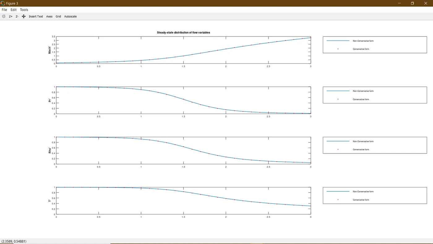
1)Steady-state distribution of primitive variables inside the nozzle:

The plots for the steady state distribuition of flow variables is similar for both conservative and Non Conservative forms at 1400 time steps which are matching with analytical solutions provided in Anderson book and the plot is as follows:

2) Time-wise variation of the primitive variables:

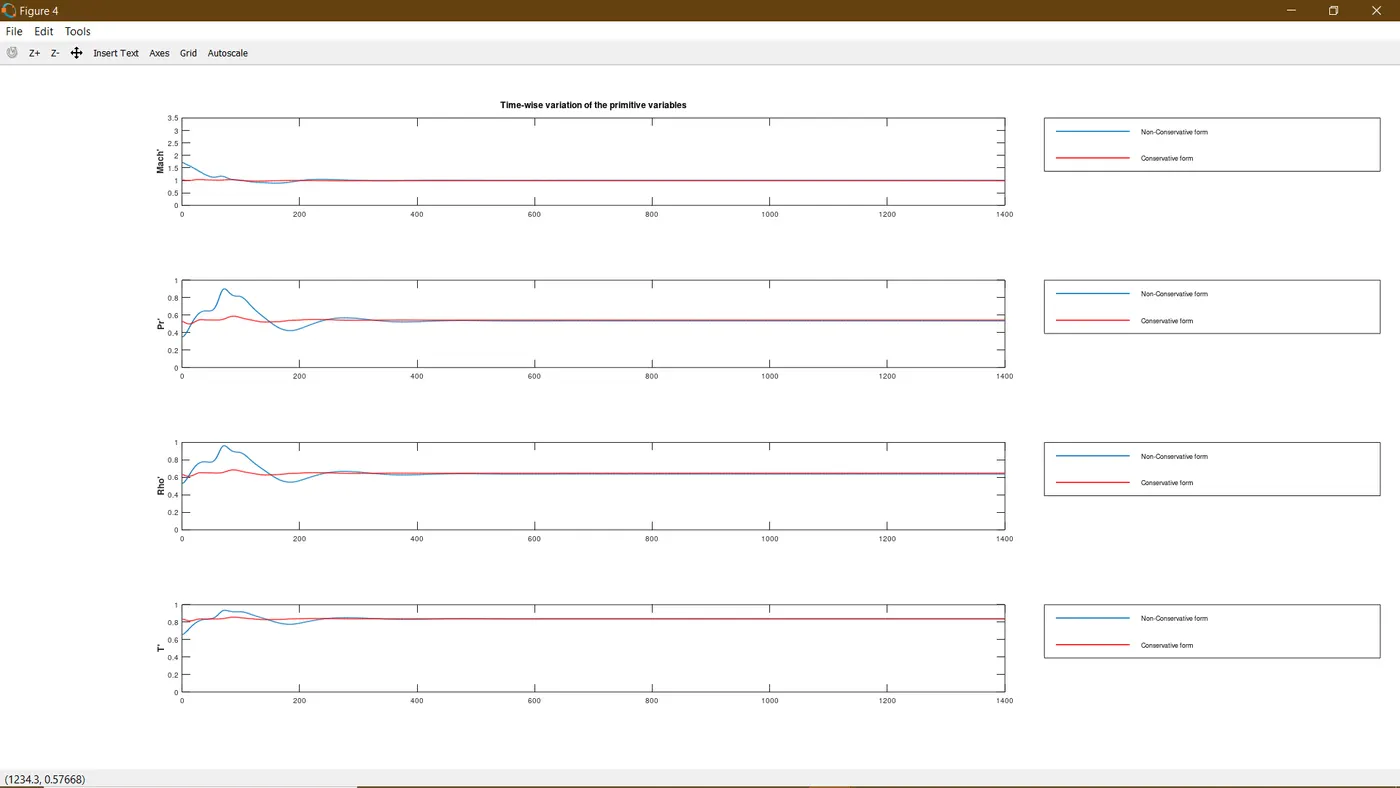
From the above plot results the following observations are noted:

a) For both forms, the steady state is acheived approximately after 500 time steps and after 700 time steps, the plots are alomst matching with exact solution with minimal error.

b) Compared to Conservative, the Non Conservative form obatained accurate values as the solutions of pressure, density and temperature are almost matching with exact solutions.

c) The behaviour of residuals for the conversation form is not as good as that for the conversation form of equations. For Non Conservation form the residual becomes low from order of 10^-1 to 10^-6 after 1400 time steps, where as for conservative decay only to 10^-3 to 10^-1.

d)By time wise variations of flow variables plot, we can easily track the values at particular timestep.

e) Non Conservative leads to smaller residue compared to Conservative because of the quality index is depends on the rate of decay of residue.

3) Variation of Mass flow rate distribution inside the nozzle at different time steps during the time-marching process:

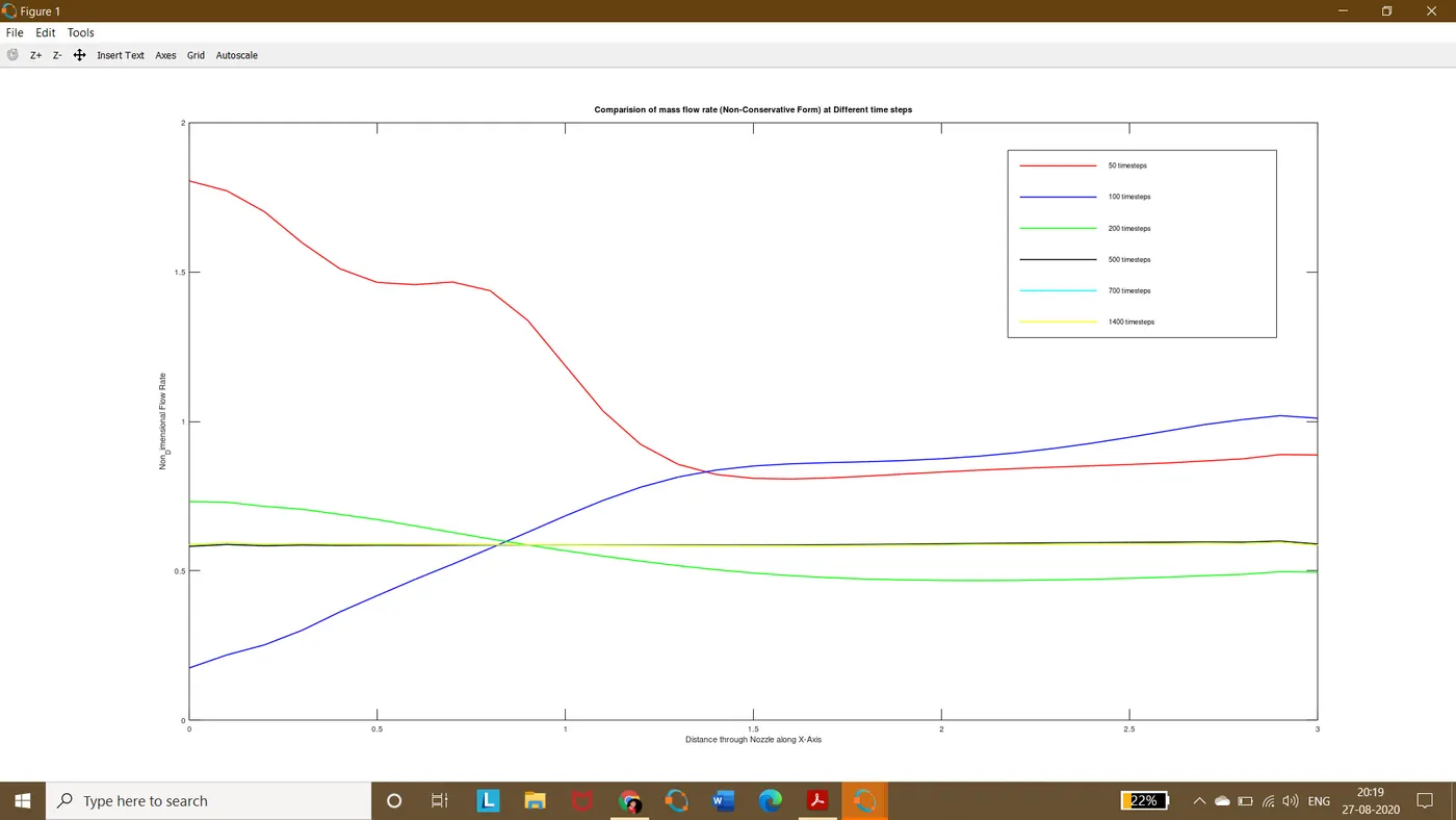
A) Non Conservative form: The timewise variation of the flow and its approach to the steady state provided by the mass flow variations shown in below figure. Six different curves are shown, each for a different time during the course of time marching process.

Observations:

1) Intially looking for 50 timesteps, the curve osciliates heavily and for 100 time steps the mass flow rate chaged radically. However after 200 timesteps, the mass flow distribution is a straight, and horizontal line across the graph.

2) After 500 and 700 time steps the flow is constant which satisfies our basic law which is pVA = constant.

3) As per the above plot, we will get the steady state around 700 timesteps itself, but for accurate results upto three decimal accuracy we are going about 1400 time steps.

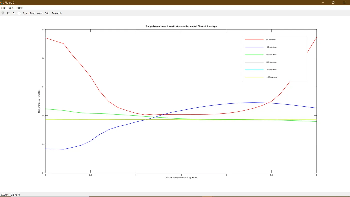
B) Conservative form:

The time wise variation of the flow same as like non conservative form, the mass flow variations are shown for conservative form are shown below. Here also we are taking six differnt plots as like above.

Observations:

1) By looking at the above plot, we can get to know that initially the curve at 50 time steps osciliates heavily but for 100 time steps it becomes some what Humped distribution.

2) After 200 time steps, the mass flow distribution becoming more constant.

3) After 500 and 700 time steps, the mass flow rate becomes approximately equals to a constant value. Moreover it is quite close to analytical value.

4) Comparison of Normalized mass flow rate distributions of both forms:

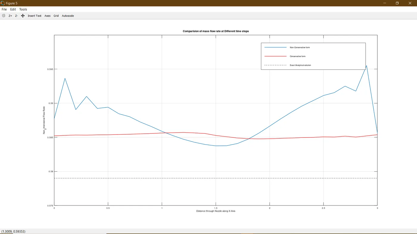
The comparision of mass flow rates for both Non conservative and conservative forms are shown in the below figure.

Observations:

a) By looking to above plot, we can come to know that the plot of conservative form is more satisfactory compared to the Non Conservative form.

b) The main reason for above statement is that the mass flow distribution is becoming more closer value to analytical solution. Where as in Non Conservative form, a small amount of variation with sharp oscillations at both inlet and outlet.

c)By seeing the red line we can come to know that the results are much closer to the analytical solution and more over the oscillations are very less compared to Non Conservative form.

The main reason behind the conversation form does a better job is that the mass flow is one of the dependant variables in the equations. Where as in Non Conservative form, the dependant variables are the primitive variables and the mass flow is obtained after the outcome of primitive variables.

GRID INDEPENDENCE TEST:

By looking the above plot and statements, we cannot come to conclude that the conversation form is more accurate and superior than non Conservative form. If we consider the primitive variables such as temperature, pressure, and mach number at nozzle thorat. The following table shows the results of both conservative and Non conservative form compared with analytical data while the number of grid points are of 31 and 61.

Primitive variables	Non- Conservative form		Conservative form		Analytical solution
	N = 31	N = 61	N = 31	N = 61
Rho	0.639	0.638	0.649	0.646	0.634
Mach	0.999	1.0	0.985	0.998	1.000
Pressure	0.534	0.532	0.544	0.534	0.528
Temperature	0.836	0.835	0.839	0.836	0.833

The last column of the above table repersents the exact analytical solution. By observing the values of second column and fourth column, the values of the Non conservative form is nearly close to the exact solution. The comparisonof the third row and fifth row ( n = 61), we can get to know that the values of conservative comes closer to the analytical solution, but in the case of non conservative form the values at n = 31 itself are closer to the eaxct values. Note that by doubling the number of grid points, the steady state results are slighty closer to the exact values, this clearly shows the indication of Grid Independence for the conversation form resuts. For alla practical purposes, we have grid independence with 31 grid points.

CONCLUSION:

As we applied both the Non Conservation form and Conservation forms for solutions of the subsonic- supersonic isentropic nozzle which is considered as Quasi 1D an compared all the results. We can comclude that the results are same for both forms, the main difference between is that the conservative form have superiority when it comes to mass flow distribution where as the Non Conservative form yeilds better values when it comes to primitve variables. And when it comes to caluculation effort to achive a solution, the conservative form takes more time than Non conservative because the values has to decode from the flux variables.