Week 3 - Adiabatic Flame Temperature calculation
Aim: Adiabatic flame temperature calculation.
Introduction:
Adiabatic flame temperature:
The final temperature that is obtained after the fuel is completely burned is called the adiabatic flame temperature.
To calculate the adiabatic flame temperature of any process, the first step is to balance the combustion equation.
The most general form is given by:
Fuel + air = products
Let us take an example with fuel as methane burning in the air-
CH4 + 2O2 => CO2 +2H2O
For any fuel with form CxHy the general form of the equation can be given as:
CxHy + (x+y/4) O2 => xCO2 + (y/2) O2
If nitrogen is also being considered in the equation then it turns to be:
CxHy + (x+y/4)*(O2+3.72N2) => xCO2 + (y/2) O2 + (x+y/4)*3.72*N2
Now we got the equation for the combustion process, in this process we assume that the reactants are burned at standard temperature and pressure (T = 298K, P=1atm)
We now have the reactant's pressure and temperature using which we can calculate the Enthalpy of formation of reactants.
There are two types of possibilities:
- Constant volume adiabatic flame temperature
- Constant pressure adiabatic flame temperature
Constant volume adiabatic flame temperature:
In this method, we use the internal energy of reactants and products with which we will calculate the adiabatic temperature.
Ureactants = Uproducts
We know that U = H - PV
Now equation in terms of enthalpy can be given as
(Hproducts - Hreactants) – V*(Pinitial - Pfinal) = 0 ---------------- (1)
From ideal gas law:
P*V = N*Ru*T
Where,
N= No of moles
Ru = universal gas constant
T = temperature Tini, and Tadiabatic
The final equation after applying ideal gas law to eq(1)
(Hproducts - Hreactants) - (Nreactants*Ru*Tinitial - Nproducts*Ru*Tadiabatic) = 0
Constant pressure adiabatic flame temperature:
The first law of thermodynamics defines this process, the equation can be simply written as.
(H_products – H_reactants) = 0
The adiabatic temperature for the constant volume process is greater than that of the constant volume method because in the constant pressure process the heat is lost because of an increase in volume.
LOWER HEATING VALUE:
The amount of energy that can be extracted from particular fuel.
Consider we have an equation as:
CH4 + 2O2 => CO2 +2H2O
At STP
LHV = h298f, CH4 + h298f, O2 - h298f, CO2 - h298f, H2O
Now if heat loss is given in the problem we can take product of heat Loss and LHV which we can add to equation to get Heat of reaction.
Equivalence ratio:
It is ratio of Fuel by Air of given mixture to Fuel by Air of stoichiometric mixture.
The equivalence ratio is denoted by symbol Ø
Ø = (F/A) given mixture / (F/A) stoichiometric mixture
If Ø>1 the mixture is rich mixture
If Ø<1 the mixture is lean mixture
If Ø=1 the mixture is stoichiometric mixture
Equation for types of mixture:
Rich mixture:
Due to greater amount of fuel then air the products side there is emission of CO and HX.
Let us take a equation and demostrate the rich mixture-
The general form for CxHy fuel with rich mixture can be written as.
Ø*CxHy +2*(O2+3.72N2) => (4 - Øy/2 - Øx) CO2 + (Øy/2) O2 + 2*3.72*N2 + (2Øx +Øy/2 -4) CO
Just the Equivalence ratio is multiplied with fuel if the value >1 the fuel is more compared to air which makes it rich.
Lean mixture:
The general form of equation after calculation is:
Ø*CxHy +2*(O2+3.72N2) => ØxCO2 + (Øy/2) O2 + 2*3.72*N2 + (2 - Øx - Øy/4) O2
How we can distinguish between this two mixtures??
Some of the basic example which we see in our daily life are, when there is less fuel in our vehicle the mixture gets lean and the vehicle get off and on again and again, and rich mixture is present when we start the engine we can guess it with knocking sound.
The table which shows us the variation of mixture with respect to torque and speed in RPM:
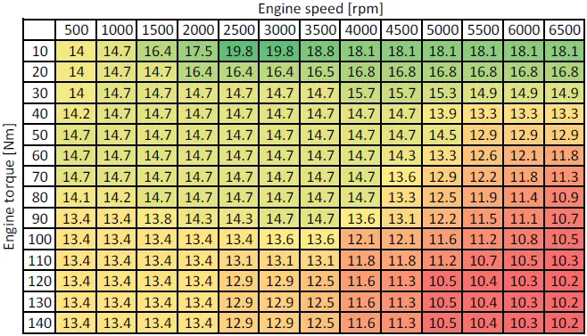
Basically for ic engine the AFR varies from range 12:1 (rich) to 20:1 (lean).
Program steps/Logic:
- Import the required modules in the python code.
- First step is to write a function for calculation of enthalpy using nasa polynomial.
- To get a values of enthalpy we should extract data from nasa thermodynamic file for required species.
- Once we got a enthalpy of formation of each species we will create a function to calculate enthalpy of formation.
- In calculating enthalpy of reaction the reactants temperature is known but the products tempearture(Adiabatic temperature) is unknown,To calculate it we will use newton raphson method.
- The last step is we can compare our python values with cantera.
- This above steps are generally applicable for all the cases which are being given as our objective.
Universal python code to solve all the objectives:
Instruction of cases:
- Case 1 = Finding adiabatic flame temperature for constant volume chamber and also plot variation of adiabatic flame temperature with respect to equivalence ratio
- Case 2 = Considering a constant pressure reactor with heat loss. The reactor is initially set at STP conditions.
The heat loss will controlled heat using a variable called H_loss.
Example, H_loss = 0.5 would mean a heat loss that is equal to 50% of the maximum possible heat loss. - Case 3 = Considering the fuel type to be of the form CxHy.
Phi and lambda = 1.0. Finding the AFT of CH4 with H_loss = 0.35
Testing it for -ane, -ene and -yne variants of 2 Carbon atom chain and plotting a trend. - Case 4 = For a general alkane, plotting the effect of the number of carbon atoms (from 1 to 3) on the final temperature. Assume H_loss = 0
import math
import matplotlib.pyplot as plt
import numpy as np
import cantera as ct

"""
adiabatic flame test
"""
# function to calculate enthalpy for reactants and product ny using nasa thermo data file
def coeff(T,coeffs):

	a1 = coeffs[0]
	a2 = coeffs[1]
	a3 = coeffs[2]
	a4 = coeffs[3]
	a5 = coeffs[4]
	a6 = coeffs[5]
	return (a1 + a2*T/2 + a3*pow(T,2)/3 + a4*pow(T,3)/4 + a5*pow(T,4)/5 +a6/T)*R*T

#value of coefficents for higher and lower temperature of species
#low temperature co-efficients reactants side
l_coeffs_ch4 = [5.14987613E+00,-1.36709788E-02, 4.91800599E-05, -4.84743026E-08, 1.66693956E-11,-1.02466476E+04]

l_coeffs_c2h6 = [4.29142492E+00,-5.50154270E-03,5.99438288E-05,-7.08466285E-08, 2.68685771E-11,-1.15222055E+04]

l_coeffs_c2h4 = [3.95920148E+00,-7.57052247E-03, 5.70990292E-05,-6.91588753E-08, 2.69884373E-11, 5.08977593E+03]

l_coeffs_c2h2 =[8.08681094E-01,2.33615629E-02,-3.55171815E-05,2.80152437E-08,-8.50072974E-12,2.64289807E+04]

l_coeffs_c3h8 = [0.93355381E+00,0.26424579E-01,0.61059727E-05,-0.21977499E-07,0.95149253E-11,-0.13958520E+05]

l_coeffs_o2 = [3.78245636E+00,-2.99673416E-03, 9.84730201E-06, -9.68129509E-09, 3.24372837E-12,-1.06394356E+03]

l_coeffs_n2 = [0.03298677E+02, 0.14082404E-02,-0.03963222E-04, 0.05641515E-07,-0.02444854E-10,-0.10208999E+04]

#higher temperature co-efficients products side
h_coeffs_n2 = [0.02926640E+02, 0.14879768E-02,-0.05684760E-05, 0.10097038E-09,-0.06753351E-13,-0.09227977E+04]

h_coeffs_o2 = [3.28253784E+00, 1.48308754E-03,-7.57966669E-07, 2.09470555E-10,-2.16717794E-14,-1.08845772E+03]

h_coeffs_co = [2.71518561E+00,2.06252743E-03,-9.98825771E-07, 2.30053008E-10,-2.03647716E-14,-1.41518724E+04]

h_coeffs_co2 = [3.85746029E+00, 4.41437026E-03,-2.21481404E-06, 5.23490188E-10,-4.72084164E-14,-4.87591660E+04]

h_coeffs_h2o = [3.03399249E+00, 2.17691804E-03,-1.64072518E-07,-9.70419870E-11, 1.68200992E-14,-3.00042971E+04]

#Inputs
Tstp = 298.15 #in kelvin
R = 8.314
alpha = 1 # relaxation factor
tol = 1e-3 #tolerance
phi = np.linspace(0.1,2,30) #equivalence factor value for calculation of adiabatic flame temperature in case 1
H_loss = np.linspace(0,1,10) # Heat loss value in case of constant pressure for calculation of adiabatic flame temperature in case 2
y = np.linspace(6,2,3) # Value to calculate Adiabatic flame temperature of alkane, alkene and alkyne
x = np.linspace(1,3,3) # Value to calculate Adiabatic flame temperature of different alkanes
H_loss_s = 0.35 # heat loss value for different species in case 3
Tad_phi = []
Tad_hloss = []
Tad_species = []
Tad_alkanes = []
itera = []            # For counting the number of iteration taken
T_guess = 1500        # initial guess of adiabatic temperature for newton raphson method

"""
DETAILS OF CASES TO BE ANALYSED:

* case 1 = Finding adiabatic flame temperature for constant volume chamber and also plot variation of adiabatic flame temperature with respect to equivalence ratio
* case 2 = Considering a constant pressure reactor with heat loss. The reactor is initially set at STP conditions.
         The heat loss will controlled heat using a variable called H_loss.
         Example, H_loss = 0.5 would mean a heat loss that is equal to 50% of the maximum possible heat loss.
* case 3 = Considering the fuel type to be of the form CxHy.
 		Phi and lambda = 1.0. Finding the AFT of CH4 with H_loss = 0.35
		Testing it for -ane, -ene and -yne variants of 2 Carbon atom chain and plotting a trend.
* case 4 = For a general alkane, plotting the effect of the number of carbon atoms (from 1 to 3) on the final temperature. Assume H_loss = 0
"""

case = input('The case to be runned = ')  # Taking input from user f
case = int(case)
if case == 1:
	#Function to return total enthalpy
	def f(T,phi):
		#reactants
		H_CH4_r = coeff(Tstp,l_coeffs_ch4)
		H_o2_r = coeff(Tstp,l_coeffs_o2)
		H_n2_r = coeff(Tstp,l_coeffs_n2)

		H_reactants = phi*H_CH4_r + 2*H_o2_r + 7.52*H_n2_r
		N_reactants = (phi + 2 + 7.52)*R*Tstp
		#products
		H_n2_p = coeff(T,h_coeffs_n2)
		H_co2_p = coeff(T,h_coeffs_co2)
		H_h2o_p = coeff(T,h_coeffs_h2o)
		H_co_p = coeff(T,h_coeffs_co)
		H_o2_p = coeff(T,h_coeffs_o2)

		if phi >= 1:
			H_products = (4-3*phi)*H_co2_p + 2*phi*H_h2o_p + 7.52*H_n2_p + (4*phi-4)*H_co_p
			N_products = ((4-3*phi) + 2*phi + (7.52) + (4*phi-4))*R*T

		elif phi < 1:
			H_products = phi*H_co2_p + 2*phi*H_h2o_p + 7.52*H_n2_p + (2-(5*phi/4))*H_o2_p
			N_products = (phi + 2*phi + 7.52 + (2-(5*phi/4)))*R*T

		return (H_products - H_reactants) - (N_products - N_reactants)

	#function for applying differencing schemes
	#central differencing scheme
	def fprime(T,phi):
		return (f(T+1e-6,phi)-f(T-1e-6,phi))/(2*1e-6)

	#Function to compute value using newton Raphson technique
	for i in range(0,len(phi)):
		iteration = 1
		while abs(f(T_guess,phi[i])) >= tol:
			T_guess = T_guess - alpha*((f(T_guess,phi[i]))/(fprime(T_guess,phi[i])))
			iteration = iteration +1
		itera.append(iteration)
		Tad_phi.append(T_guess)
	print(Tad_phi)
	print(itera)
	"""
	Cantera
	"""
	Tad_ct = []
	gas = ct.Solution('gri30.xml')

	for i in range(0,len(phi)):
		#calculating the mole fraction of reactants to use in equation
		N_total = 1+(2/phi[i])+(7.32/phi[i])
		N_CH4 = 1/N_total
		N_O2 =(2/phi[i])/(N_total)
		N_N2 = (7.32/phi[i])/(N_total)
		gas.TPX = 298.15,101325,{'CH4':N_CH4 , 'O2':N_O2, 'N2':N_N2}
		gas.equilibrate('HP','auto')
		Tad_ct.append(gas.T)

	#Plotting
	plt.title('Equivalence factor VS Adiabatic flame temperature')
	plt.plot(phi,Tad_ct,'o-',color='r')
	plt.plot(phi,Tad_phi,'o-',color='b')
	plt.xlabel('Equivalence factor')
	plt.ylabel('Adiabatic flame temperature')
	plt.legend(["AFT cantera","AFT python"], loc = 'best')
	plt.show()

	#CASE END


elif case == 2:
	#Function to return total enthalpy
	def f(T,H_loss):
		#reactants
		H_CH4_r = coeff(Tstp,l_coeffs_ch4)
		H_o2_r = coeff(Tstp,l_coeffs_o2)
		H_n2_r = coeff(Tstp,l_coeffs_n2)

		H_reactants = H_CH4_r + 2*H_o2_r + 7.52*H_n2_r
		#products
		H_n2_p_stp = coeff(Tstp,h_coeffs_n2)
		H_co2_p_stp = coeff(Tstp,h_coeffs_co2)
		H_h2o_p_stp = coeff(Tstp,h_coeffs_h2o)

		H_n2_p = coeff(T,h_coeffs_n2)
		H_co2_p = coeff(T,h_coeffs_co2)
		H_h2o_p = coeff(T,h_coeffs_h2o)

		H_products = H_co2_p + 2*H_h2o_p + 7.52*H_n2_p
		LHV = H_CH4_r + 2*H_o2_r - H_co2_p_stp - 2*H_h2o_p_stp

		return H_products - H_reactants +(H_loss*LHV)

	#function for applying differencing schemes
	#central differencing scheme
	def fprime(T,H_loss):
		return (f(T+1e-6,H_loss)-f(T-1e-6,H_loss))/(2*1e-6)

	#Function to compute value using newton Raphson technique
	for i in range(0,len(H_loss)):
		iteration = 1
		while abs(f(T_guess,H_loss[i])) >= tol:
			T_guess = T_guess - alpha*((f(T_guess,H_loss[i]))/(fprime(T_guess,H_loss[i])))
			iteration = iteration +1
		itera.append(iteration)
		Tad_hloss.append(T_guess)
	print(Tad_hloss)
	print(itera)

	plt.plot(H_loss,Tad_hloss,'o-r')
	plt.title('Heat loss vs adiabatic flame temperature')
	plt.xlabel('Heat loss')
	plt.ylabel('Adiabatic flame temperature')
	plt.show()

	#CASE END


elif case ==3:
	#Function to return total enthalpy
	def f(T,y):
		#reactants at stp

		H_o2_r = coeff(Tstp,l_coeffs_o2)
		H_n2_r = coeff(Tstp,l_coeffs_n2)
		#products at stp
		H_n2_p_stp= coeff(Tstp,h_coeffs_n2)
		H_co2_p_stp = coeff(Tstp,h_coeffs_co2)
		H_h2o_p_stp = coeff(Tstp,h_coeffs_h2o)

		#products at adiabatic temperature
		H_n2_p_ad = coeff(T,h_coeffs_n2)
		H_co2_p_ad = coeff(T,h_coeffs_co2)
		H_h2o_p_ad = coeff(T,h_coeffs_h2o)

		if y == 6:
			H_C2H6_r = coeff(Tstp,l_coeffs_c2h6)
			H_r_stp = H_C2H6_r + 3.5*H_o2_r + 3.5*3.72*H_n2_r
			H_prod_stp = 2*H_co2_p_stp + 3*H_h2o_p_stp + 3.5*3.72*H_n2_p_stp
			H_prod_Tad = 2*H_co2_p_ad + 3*H_h2o_p_ad + 3.5*3.72*H_n2_p_ad
		elif y == 4:
			H_C2H4_r = coeff(Tstp,l_coeffs_c2h4)
			H_r_stp = H_C2H4_r + 3*H_o2_r + 3*3.72*H_n2_r
			H_prod_stp = 2*H_co2_p_stp + 2*H_h2o_p_stp + 3*3.72*H_n2_p_stp
			H_prod_Tad = 2*H_co2_p_ad + 2*H_h2o_p_ad + 3*3.72*H_n2_p_ad
		else:
			H_C2H2_r = coeff(Tstp,l_coeffs_c2h2)
			H_r_stp = H_C2H2_r + 2.5*H_o2_r + 2.5*3.72*H_n2_r
			H_prod_stp = 2*H_co2_p_stp + H_h2o_p_stp + 2.5*3.72*H_n2_p_stp
			H_prod_Tad = 2*H_co2_p_ad + H_h2o_p_ad + 2.5*3.72*H_n2_p_ad


		LHV = H_r_stp - H_prod_stp

		return H_prod_Tad - H_r_stp +(H_loss_s*LHV)

	#function for applying differencing schemes
	#central differencing scheme
	def fprime(T,y):
		return (f(T+1e-6,y)-f(T-1e-6,y))/(2*1e-6)

	#Function to compute value using newton Raphson technique
	for i in range(0,len(y)):
		iteration = 1
		while abs(f(T_guess,y[i])) >= tol:
			T_guess = T_guess - alpha*((f(T_guess,y[i]))/(fprime(T_guess,y[i])))
			iteration = iteration +1
		itera.append(iteration)
		Tad_species.append(T_guess)
	print(Tad_species)
	print(itera)

	x = ["alkane","alkene","alkyne"]
	plt.barh(x,Tad_species)
	plt.title('Adiabatic flame temperature for different species')
	plt.show()

	#CASE END

elif case==4:
	#Function to return total enthalpy
	def f(T,x):
		#reactants at stp
		H_o2_r = coeff(Tstp,l_coeffs_o2)
		H_n2_r = coeff(Tstp,l_coeffs_n2)

		#products at adiabatic temperature
		H_n2_p_ad = coeff(T,h_coeffs_n2)
		H_co2_p_ad = coeff(T,h_coeffs_co2)
		H_h2o_p_ad = coeff(T,h_coeffs_h2o)

		if x == 1:
			H_CH4_r = coeff(Tstp,l_coeffs_ch4)
			H_r_stp = H_CH4_r + 2*H_o2_r + 7.52*H_n2_r
			H_prod_Tad = H_co2_p_ad + 2*H_h2o_p_ad + 7.52*H_n2_p_ad
		elif x == 2:
			H_C2H6_r = coeff(Tstp,l_coeffs_c2h6)
			H_r_stp = H_C2H6_r + 3.5*H_o2_r + 3.5*3.72*H_n2_r
			H_prod_Tad = 2*H_co2_p_ad + 3*H_h2o_p_ad + 3.5*3.72*H_n2_p_ad
		else:
			H_C3H8_r = coeff(Tstp,l_coeffs_c3h8)
			H_r_stp = H_C3H8_r + 5*H_o2_r + 5*3.72*H_n2_r
			H_prod_Tad = 3*H_co2_p_ad + 4*H_h2o_p_ad + 5*3.72*H_n2_p_ad


		return H_prod_Tad - H_r_stp
	#function for applying differencing schemes
	#central differencing scheme
	def fprime(T,y):
		return (f(T+1e-6,y)-f(T-1e-6,y))/(2*1e-6)

	#Function to compute value using newton Raphson technique
	for i in range(0,len(x)):
		iteration = 1
		while abs(f(T_guess,x[i])) >= tol:
			T_guess = T_guess - alpha*((f(T_guess,x[i]))/(fprime(T_guess,x[i])))
			iteration = iteration +1
		itera.append(iteration)
		Tad_alkanes.append(T_guess)
	print(Tad_alkanes)
	print(itera)

	x = np.array(["Methane","Ethane","Propane"])
	plt.barh(x,Tad_alkanes)
	plt.title('Adiabatic flame temperature for different Alkanes')
	plt.show()

	#CASE END
Plots -
CASE :1
The variation of adiabatic flame temperature with equivalence ratio for python and cantera.
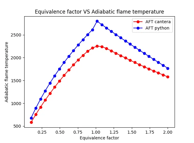
From the plot its is seen that the cantera provides lower temperature which is more accurate the python code.
The reason is in cantera the file gri30.cti consists of may products which we have not included in python code which makes difference in AFT value.
CASE :2
The variation of adiabatic flame temperature with heat loss.
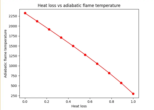
In this plot it can be seen as the Heat loss value goes from 0 to 100% the value of adiabatic flame temperature goes on decreasing and at 100% Heat loss the value for AFT of products is same as reactants(STP).
CASE :3
The variation of adiabatic flame temperature with alkane,alkene, and alkyne(ethane,ethene and ethyne).
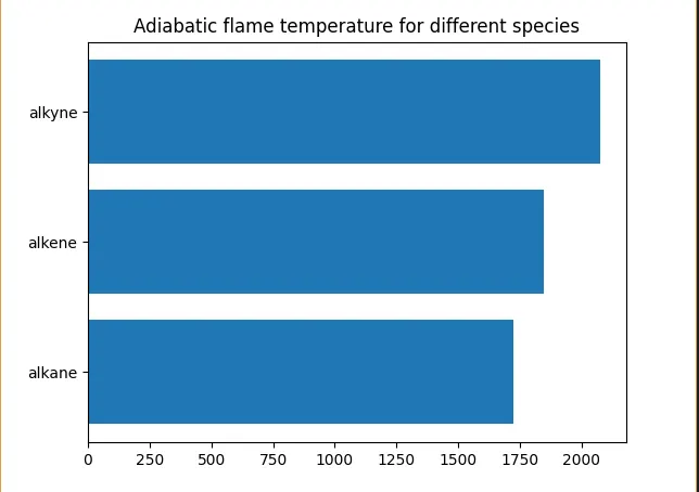
The above plot shows that the excess hydrogen will give a greater adiabatic flame temperature,The study shows that adding hydrogen can improve the combustion efficiency of engines.Also considerable reduction in
UHC and other pollutants from 56 ppm to the lowest value (31 ppm) at higher hydrogen fractions.
CASE :4
The variation of adiabatic flame temperature with alkanes
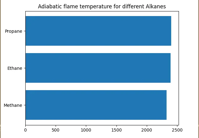
As we know from above plot in case 3 that increase in hydrogen atoms increase the adiabatic flame temperature is base for this case which provides an idea that alkane of higher order will have greater adiabatic flame temperature. The difference in temperature is smaller since carbon number also increases with somewhat try to balance a effect.
Bibilography:
https://en.wikipedia.org/wiki/Adiabatic_flame_temperature
An introduction to combustion by - Stephen R Turns