Derivation and Plotting the Errors for a Fourth Order Approximation for a Second Order Derivative using the Taylors Table.
Week 3 Report.
- Aim: To derive the following 4th order approximations of the second-order derivative
a. Central Differencing.
b. Skewed Left Sided Difference.
c. Skewed Right Sided Difference. - Theoretical Introduction:
In mathematics, the Taylor series of a function is an infinite sum of terms that are expressed in terms of the function's derivatives at a single point. For most common functions, the function and the sum of its Taylor series are equal near this point. Taylor's series are named after Brook Taylor who introduced them in 1715.
If zero is the point where the derivatives are considered, a Taylor series is also called a Maclaurin series, after Colin Maclaurin, who made extensive use of this special case of Taylor series in the 18th century.
The partial sum formed by the first n + 1 terms of a Taylor series is a polynomial of degree n that is called the nth Taylor polynomial of the function. Taylor polynomials are approximations of a function, which become generally better as n increases. Taylor's theorem gives quantitative estimates on the error introduced by the use of such approximations. If the Taylor series of a function is convergent, its sum is the limit of the infinite sequence of the Taylor polynomials. A function may differ from the sum of its Taylor series, even if its Taylor series is convergent. A function is analytic at a point x if it is equal to the sum of its Taylor series in some open interval (or open disk in the complex plane) containing x. This implies that the function is analytic at every point of the interval (or disk).
Formulation:
The Taylor series of a real or complex-valued function f (x) that is infinitely differentiable at a real or complex number a is the power series
where n! denotes the factorial of n. In the more compact sigma notation, this can be written as
where f(n)(a) denotes the nth derivative of f evaluated at the point a. (The derivative of order zero of f is defined to be f itself and (x − a)0 and 0! are both defined to be 1.)
When a = 0, the series is also called a Maclaurin series.
We generally calculate the Differences when we want to find the approximate value for a function at a particular point. Three basic types are commonly considered: forward, backward, and central finite differences.
A forward difference is an expression of the form
Depending on the application, the spacing h may be variable or constant. When omitted, h is taken to be 1: Δ[ f ](x) = Δ1[ f ](x).
A backward difference uses the function values at x and x − h, instead of the values at x + h and x:
Finally, the central difference is given by
These are the basic types of Differences we can calculate, on the functions. The relation with the derivatives of these functions will be different.
The derivative of a function f at a point x is defined by the limit.
If h has a fixed (non-zero) value instead of approaching zero, then the Right-hand side of the above equation would be written
Hence, the forward difference divided by h approximates the derivative when h is small. The error in this approximation can be derived from Taylor's theorem. Assuming that f is differentiable, we have
The same formula holds for the backward difference:
However, the central difference yields a more accurate approximation. If f is twice differentiable,
For Higher Order Derivatives
- Second-order central

- Second order forward

- Second order backward

- Derivations:
In this, we will see the entire process of deriving these equations with basic formulae and assumptions:
Before we begin the Derivation, we must keep in mind the thumb rule for calculating the Number of points required, that is:
i) The order of accuracy P = Number of nodes in the stencil N - order of derivative Q + 1 (for symmetric/central schemes)
ii) The order of accuracy P = Number of nodes in the stencil N - order of derivative Q (for one-sided/skewed schemes)
a. For a Skewed Right sided Difference
From the above given Thumb rule, P=4, Q=2, and since this is a Skewed scheme, we use the second formula and calculate the number of points to be N=6.
The points will be:
i, i+1, i+2, i+3, i+4, i+5 with a constant difference of dx between them.
Next, we must define the second order derivative to be
`(del^2f)/(delx^2) = a*f(i) + b*f(i+1) + c*f(i+2) + d*f(i+3) + e*f(i+4) + g*f(i+5)`----------------Eq(1)
Here, we have defined a general second order derivative in terms of a Skewed Right sided System. Here, a,b,c,d,e,g are simple coefficients that we have used to describe the equation.
In the next step, we then put the Taylors Series to each and every term with respect to the first term, i.e. f(i).
`f(i+1)= f(i)+trianglex* f^'(i)/(1!)+ trianglex^2* f^('')(i)/(2!)+ trianglex^3* f^(''')(i)/(3!)+ trianglex^4* f^(iv)(i)/(4!)+ trianglex* f^(v)(i)/(5!)`
Similarly, we will calculate for the rest of the terms as well:
`f(i+2) = f(i) +(2trianglex)/(1!) * f^'(i) + (2trianglex)^2/(2!) * f^('')(i) + (2trianglex)^3/(3!) * f^(''')(i)+ (2trianglex)^4/(4!) * f^(iv)(i) + (2trianglex)^5/(5!) * f^(v)(i)`
`f(i+3) = f(i) + (3trianglex)/(1!) * f^'(i) + (3trianglex)^2/(2!) * f^('')(i) + (3trianglex)^3/(3!) * f^(''')(i)+ (3trianglex)^4/(4!) * f^(iv) + (3trianglex)^5/(5!) * f^(v)(i)`
`f(i+4) = f(i) + (4trianglex)/(1!)*f^(')(i)+ (4trianglex)^2/(2!)*f^('')(i)+ (4trianglex)^3/(3!)*f^(''')(i)+ (4trianglex)^4/(4!)*f^(iv)(i)+ (4trianglex)^5/(5!)*f^(v)(i)`
`f(i+5) = f(i) + (5trianglex)/(1!)*f^(')(i)+ (5trianglex)^2/(2!)*f^('')(i)+ (5trianglex)^3/(3!)*f^(''')(i)+ (5trianglex)^4/(4!)*f^(iv)(i)+ (5trianglex)^5/(5!)*f^(v)(i)`
In the next step, we will multiply the coefficients with the respective terms form equation(1):
`a*f(i)`
`b*f(i+1)= b*f(i)+b*trianglex* f^'(i)/(1!)+ b* trianglex^2* f^('')(i)/(2!)+ b*trianglex^3* f^(''')(i)/(3!)+ b*trianglex^4* f^(iv)(i)/(4!)+ b*trianglex* f^(v)(i)/(5!)`
`c* f(i+2) = c*f(i) +c*(2trianglex)/(1!) * f^'(i) + c*(2trianglex)^2/(2!) * f^('')(i) + c*(2trianglex)^3/(3!) * f^(''')(i)+ c*(2trianglex)^4/(4!) * f^(iv)(i)`
+ `c*(2trianglex)^5/(5!) * f^(v)(i)`
`d*f(i+3) = d*f(i) + d*(3trianglex)/(1!) * f^'(i) + d*(3trianglex)^2/(2!) * f^('')(i) + d*(3trianglex)^3/(3!) * f^(''')(i)+ d*(3trianglex)^4/(4!) * f^(iv)`
+ `d*(3trianglex)^5/(5!) * f^(v)(i)`
`e*f(i+4) = e*f(i) + e*(4trianglex)/(1!)*f^(')(i)+ e*(4trianglex)^2/(2!)*f^('')(i)+ e*(4trianglex)^3/(3!)*f^(''')(i)+ e*(4trianglex)^4/(4!)*f^(iv)(i)`
+ `e*(4trianglex)^5/(5!)*f^(v)(i)`
`g*f(i+5) = g*f(i) + g*(5trianglex)/(1!)*f^(')(i)+ g*(5trianglex)^2/(2!)*f^('')(i)+ g*(5trianglex)^3/(3!)*f^(''')(i)+ g*(5trianglex)^4/(4!)*f^(iv)(i)`
+ `g*(5trianglex)^5/(5!)*f^(v)(i)`
Next, we must club all the similar terms as shown below:
= `f(i) [a+b+c+d+e+g] `
+ `f^(')(i) [b*(trianglex)/(1!)+ 2c*(trianglex)/(1!)+ 3d*(trianglex)/(1!)+ 4e*(trianglex)/(1!)+5g*(trianglex)/(1!)]`
+ `f^('')(i)[b*(trianglex)^2/(2!)+ c*(2trianglex)^2/(2!)+ d*(3trianglex)^2/(2!)+ e*(4trianglex)^2/(2!)+ g*(5trianglex)^2/(2!)]`
+ `f^(''')(i) [b*(trianglex)^3/(3!)+ c*(2trianglex)^3/(3!)+ d*(3trianglex)^3/(3!)+ e*(4trianglex)^3/(3!)+ g*(5trianglex)^3/(3!)]`
+ `f^(iv)(i) = [b*(trianglex)^4/(4!)+ c*(2trianglex)^4/(4!)+ d*(3trianglex)^4/(4!)+ e*(4trianglex)^4/(4!)+ g*(5trianglex)^4/(4!)]`
+ `f^(v)(i) = [b*(trianglex)^5/(5!)+ c*(2trianglex)^5/(5!)+ d*(3trianglex)^5/(5!)+ e*(4trianglex)^5/(5!)+ g*(5trianglex)^5/(5!)]`
We get the following Equations as follows:
a+b+c+d+e+g = 0
b+2c+3d+4e+5g = 0
b+4c+9d+16e+25g = 2 (We keep this variable as 1 because its a second order derivative and this variable represents the second order derivative of the function)
b+8c+27d+64e+125g = 0
b+16c+81d+256e+625g = 0
b+ 32c+243d+1024e+3125g =0
From the Above equations, we see that we have six variables and we need six equations to solve for them. We must use these equations to then calculate the unknown variables, those are: a,b,c,d,e,g. We can use MATLAB to then use the Matrix inversion to calculate them.
So, We define the Matrices as the following:
A1= `[[1,1,1,1,1,1],[ 0,1,2,3,4,5], [0,1,4,9,16,25],[0,1,8,27,64,125],[0,1,16,81,256,625],[0,1,32,243,1024,3125]]`
X1 = `[[a] ,[b],[c],[d],[e],[g]]`
B1=`[[0],[0],[2],[0],[0],[0]]`
Then to use the Matrix inversion property, we simply put the below code and get the values of the variables.
X1=A1B1
The values of the variables are:
a= 3.7500
b= -12.8333
c= 17.8333
d= -13.0000
e= 5.0833
f= -0.8333
From the Above Equations, we get the Taylors Table for the Skewed Right Sided Difference method
| f(i) | f'(i) | f''(i) | `f^(''')(i)` | `f^(iv)(i)` | `f^(v)(i)` | |
| f(i) | a | 0 | 0 | 0 | 0 | 0 |
| f(i+1) | b | b | b | b | b | b |
| f(i+2) | c | 2c | 4c | 8c | 16c | 32c |
| f(i+3) | d | 3d | 9d | 27d | 81d | 243d |
| f(i+4) | e | 4e | 16e | 64e | 256e | 1024e |
| f(i+5) | g | 5g | 25g | 125g | 625g | 3125g |
So, the Final Fourth Order Right Sided approximation of a Second Order Derivative will be will be as follows:
`(del^2f)/(delx^2) = (3.75*f(x) - 12.8333*f(x+dx) + 17.8333*f(x+2dx) -13.0*f(x+3dx)+ 5.0833*f(x+4dx)-0.8333*f(x+5dx)) / (dx)^2`
b.For a Skewed Left sided Difference
Performing a similar derivation on the left sided difference, we get the following Equations:
a+b+c+d+e+g = 0
-b-2c-3d-4e-5g = 0
b+4c+9d+16e+25g = 2 (We keep this variable as 1 because its a second order derivative and this variable represents the second order derivative of the function)
-b-8c-27d-64e-125g = 0
b+16c+81d+256e+625g = 0
-b-32c-243d-1024e-3125g =0
Forming Matrices from the Equations above, we get
A2= `[[1,1,1,1,1,1],[ 0,-1,-2,-3,-4,-5], [0,1,4,9,16,25],[0,-1,-8,-27,-64,-125],[0,1,16,81,256,625],[0,-1,-32,-243,-1024,-3125]]`
X2 = `[[a] ,[b],[c],[d],[e],[g]]`
B2= `[[0],[0],[2],[0],[0],[0]]`
Performing Matrix Inversion, X2=A2B2, we get the following values for the coefficients:
a= 3.7500
b= -12.8333
c= 17.8333
d= -13.0000
e= 5.0833
f= -0.8333
From the Above Equations, we get the Taylors Table for the Skewed Left Sided Difference method
| f(i) | f'(i) | f''(i) | `f^(''')(i)` | `f^(iv)(i)` | `f^(v)(i)` | |
| f(i) | a | 0 | 0 | 0 | 0 | 0 |
| f(i-1) | b | -b | b | -b | b | -b |
| f(i-2) | c | -2c | 4c | -8c | 16c | -32c |
| f(i-3) | d | -3d | 9d | -27d | 81d | 243d |
| f(i-4) | e | -4e | 16e | -64e | 256e | -1024e |
| f(i-5) | g | -5g | 25g | -125g | 625g | -3125g |
So, the Final Fourth Order Left hand Sided Approximation of a Second Order Derivative will be as follows:
`(del^2f)/(delx^2) = (3.75*f(x) - 12.8333*f(x-dx) + 17.8333*f(x-2dx) -13.0*f(x-3dx)+ 5.0833*f(x-4dx)-0.8333*f(x-5dx)) / (dx)^2`
c. For Central Differencing
Performing a similar derivation on the left sided difference, we get the following Equations:
a+b+c+d+e = 0
-2a-b+d+2e = 0
4a+b+d+4e = 2 (We keep this variable as 1 because its a second order derivative and this variable represents the second order derivative of the function)
-8a-b+d+8e = 0
16a+b+d+16e = 0
Forming Matrices from the Equations above, we get,
A3= `[[1,1,1,1,1],[-2,-1,0,1,2],[4,1,0,1,4],[-8,-1,0,1,8],[16,1,0,1,16]]`
X3 = `[[a] ,[b],[c],[d],[e]]`
B3= `[[0],[0],[2],[0],[0],[0]]`
Performing Matrix Inversion, X3=A3B3, we get the following values for the coefficients:
a= -0.0833
b= 1.3333
c= -2.5000
d= 1.3333
e= -0.0833
From the Above Equations, we get the Taylors Table for the Skewed Left Sided Difference method
| f(i) | f'(i) | f''(i) | `f^(''')(i)` | `f^(iv)(i)` | `f^(v)(i)` | |
| f(i-2) | a | -2a | 4a | -8a | 16a | -32a |
| f(i-1) | b | -b | b | -b | b | -b |
| f(i) | c | 0 | 0 | 0 | 0 | 0 |
| f(i+1) | d | d | d | d | d | d |
| f(i+2) | e | 2e | 4e | 8e | 16e | 32e |
So, the Final Equation for the Central Difference Approximation of a Second Order Derivative will be:
`(del^2f)/(delx^2) = (-0.0833*f(x-2dx) + 1.3333*f(x-dx) - 2.5*f(x) + 1.333*f(x+dx)-0.0833*f(x+2dx)) / (dx)^2`
- Main Code:
So, the main code consists the Analytical Derivative taken as well. The Analytical derivative of the function is shown below:
`f(x) = e^(x) * cos(x)`
Analytical Derivative: `(del^2f)/(delx^2) = -2*e^x*sin(x)`
We must calculate the Analytical Derivative for all the values of dx and x and then calculate the errors for all the approximations. Then, we must later plot the graphs for them as well.
The Error can be computed using the formula shown: abs(Analytical Value- Approximated Value)
clear all close all clc %Inputs x=pi/3; dx=linspace(pi/40,pi/4000,20); %Skewed Right Hand Side A1 = [1,1,1,1,1,1; 0,1,2,3,4,5; 0,1,4,9,16,25; 0,1,8,27,64,125; 0,1,16,81,256,625; 0,1,32,243,1024,3125]; B1= [0;0;2;0;0;0]; X1= A1B1 %Divide the values of X1 by dx^2 to get the proper coefficients %Coeffs_SRH= X1/(dx)^2 %Skewed Left Hand side System A2 = [1,1,1,1,1,1; 0,-1,-2,-3,-4,-5; 0,1,4,9,16,25; 0,-1,-8,-27,-64,-125; 0,1,16,81,256,625; 0,-1,-32,-243,-1024,-3125]; B2= [0;0;2;0;0;0]; X2= A2B2 %Coeffs_SLH= X2/(dx)^2 %Central Differencing System: A3 = [1,1,1,1,1; -2,-1,0,1,2; 4,1,0,1,4; -8,-1,0,1,8; 16,1,0,1,16]; B3 = [0;0;2;0;0]; X3 = A3B3 f = exp(x)*cos(x); %Defining the function analytical_derivarive = -2*exp(x)*sin(x); %Second Order derivative for the function %Skewed right Hand side Difference Function left_hand_derivative = (X1(1)*(exp(x)*cos(x)) +(X1(2)*exp(x-dx).*cos(x-dx)) + (X1(3)*(exp(x-2*dx).*cos(x-2*dx))) + (X1(4)*(exp(x-3*dx).*cos(x-3*dx))) + (X1(5)*(exp(x-4*dx).*cos(x-4*dx))) + (X1(6)*(exp(x-5*dx).*cos(x-5*dx))))./dx.^2 right_hand_derivative = (X2(1)*(exp(x)*cos(x)) + (X2(2)*(exp(x+dx).*cos(x+dx))) + (X2(3)*(exp(x+2*dx).*cos(x+2*dx))) + (X2(4)*(exp(x+3*dx).*cos(x+3*dx))) + (X2(5)*(exp(x+4*dx).*cos(x+4*dx))) + (X2(6)*(exp(x+5*dx).*cos(x+5*dx))))./dx.^2 central_differencing = (X3(1)*exp(x-2*dx).*cos(x-2*dx) + (X3(2)*exp(x-dx).*cos(x-dx)) + (X3(3)*exp(x)*cos(x)) + (X3(4)*exp(x+dx).*cos(x+dx)) + (X3(5)*exp(x+2*dx).*cos(x+2*dx)))./dx.^2 %Plotting Results error_LHD= abs(analytical_derivarive - left_hand_derivative) error_RHD= abs(analytical_derivarive - right_hand_derivative) error_CD= abs(analytical_derivarive - central_differencing) loglog(dx,error_LHD, dx, error_RHD, dx, error_CD) xlabel('Dx') ylabel('Error for the Different types of Approximations') legend('LHD','RHD','CD','location','northwest') %End - Results:
After Plotting a graph between the error and the dx values, we get the following graph: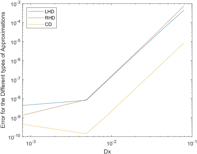
Error vs Dx Graph.
As we can see that the error that we get has a peak of somewhere in the range of 0.0001 which indicates that the accuracy of the approximation is pretty high.
The Range in which we get the error is minimum for the Central differencing method. The Accuracy is high because, in the case of a general flow, the information will be flowing in from both the directions, that is from the right hand side as well as the left hand side.
The Accuracy for the Skewed Right Hand Derivative Approximation and the Left Hand Derivative is almost the same. As we increase the value of dx, the Error occuring in the Derivative Approximation will increase thereby decreasing the Accuracy. This holds true for the Central Differencing Method as well.
- Conclusion: In conclusion I would like to state that this challenge helped me gain a better understanding on the method to extract any order approximation for any order of derivative.