Week 3.5 - Deriving 4th order approximation of a 2nd order derivative using Taylor Table method

Aim:

To derive the fourth order approximations of the second order derivative for

1. Central difference
2. Skewed right-sided difference
3. Skewed left-sided difference

Objective:

• To find the analytical solution for the function = exp(x)*cos(x)
• To calculate the error as the absolute difference between analytical solution and numerical solution
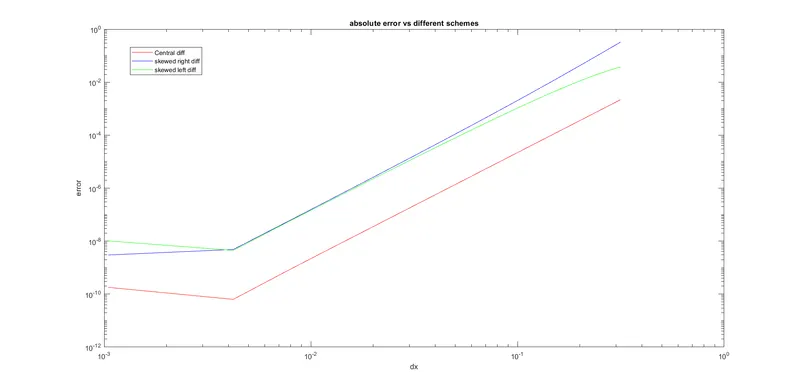
• To plot and compare error vs the different types of approximation

Theory:

Central Difference:

In this approximation the stencil is symmetric and values are taken from both the sides

To find the number of nodes in stencil:

`N=P+Q-1` where P is the order of accuracy and Q is the order of derivative

So we get ,

`N=4+2-1=5`

Therefore the hypothesis equation will be

`(del^2f)/dx^2=a*f(i-2)+b*f(i-1)+c*f(i)+d*f(i+1)+e*f(i+2)`

Using Taylor's table we get :

	`f(i)`	`trianglex*f'(i)`	`trianglex^2*f''(i)`	`trianglex^3*f'''(i)`	`trianglex^4*f''''(i)`
`a*f(i-2)`	a	-2a	4a/2	-8a/6	16a/24
`b*f(i-1)`	b	-b	b/2	-b/6	b/24
`c*f(i)`	c	0	0	0	0
`d*f(i+1)`	d	d	d/2	d/6	d/24
`e*f(i+2)`	e	2e	4e/2	8e/6	16e/24
`sum`	0	0	1	0	0

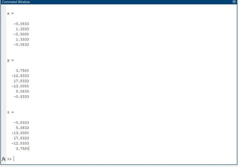
By solving the above 5 equations using matrix inversion method in MATLAB we get:

a=-0.0833
b=1.3333
c=-2.5000
d=1.3333
e=-0.0833

To find the order of accuracy :

`P=N-Q+1` since it is symmetric

where P is the order of accuracy, Q is the order of derivative and N is the number of nodes

by substituting the values,

`P=5-2+1=4`

hence order of accuracy is 4

Skewed right sided difference:

In this approximation the stencil is not symmetric and the values are only taken from right side

To find the number of nodes in stencil:

`N=P+Q` where P is the order of accuracy and Q is the order of derivative`

So we get ,

`N=4+2=6`

Therefore the hypothesis equation will be

`(del^2f)/dx^2=a*f(i)+b*f(i+1)+c*f(i+2)+d*f(i+3)+e*f(i+4)+f*f(i+5)`

Using Taylor's table we get :

	`f(i)`	`trianglex*f'(i)`	`trianglex^2*f''(i)`	`trianglex^3*f'''(i)`	`trianglex^4*f''''(i)`	`trianglex^5*f'''''(i)`
`a*f(i)`	a	0	0	0	0	0
`b*f(i+1)`	b	b	b/2	b/6	b/24	b/120
`c*f(i+2)`	c	2c	4c/2	8c/6	12c/24	32c/120
`d*f(i+3)`	d	3d	9d/2	27d/6	81d/24	243d/120
`e*f(i+4)`	e	4e	16e/2	64e/6	256e/24	1024e/120
`f*f(i+5)`	f	5f	25f/2	125f/6	625f/24	3125f/120
`sum`	0	0	1	0	0	0

By solving the above 6 equations using matrix inversion method in MATLAB we get:

a=3.7500
b=-12.8333
c=17.8333
d=-13.0000
e=5.0833
f=-0.8333

To find the order of accuracy :

`P=N-Q` since it is skewed

where P is the order of accuracy, Q is the order of derivative and N is the number of nodes

by substituting the values,

`P=6-2=4`

hence order of accuracy is 4

Skewed left sided difference:

In this approximation the stencil is not symmetric and the values are only taken from left side

To find the number of nodes in stencil:

`N=P+Q` where P is the order of accuracy and Q is the order of derivative`

So we get ,

`N=4+2=6`

Therefore the hypothesis equation will be

`(del^2f)/dx^2=a*f(i-5)+b*f(i-4)+c*f(i-3)+d*f(i-2)+e*f(i-1)+f*f(i)`

Using Taylor's table we get :

	`f(i)`	`trianglex*f'(i)`	`trianglex^2*f''(i)`	`trianglex^3*f'''(i)`	`trianglex^4*f''''(i)`	`trianglex^5*f'''''(i)`
`a*f(i-5)`	a	-5a	25a/2	-125a/6	625a/24	-3125a/120
`b*f(i-4)`	b	-4b	16b/2	-64b/6	256b/24	-1024b/120
`c*f(i-3)`	c	-3c	9c/2	-27c/6	81c/24	-243c/120
`d*f(i-2)`	d	-2d	4d/2	-8d/6	16d/24	-32d/120
`e*f(i-1)`	e	-e	e/2	-e/6	e/24	-e/120
`f*f(i)`	f	0	0	0	0	0
`sum`	0	0	1	0	0	0

By solving the above 6 equations using matrix inversion method in MATLAB we get:

a=-0.8333
b=5.0833
c=-13.0000
d=17.8333
e=-12.8333
f=3.7500

To find the order of accuracy :

`P=N-Q` since it is skewed

where P is the order of accuracy, Q is the order of derivative and N is the number of nodes

by substituting the values,

`P=6-2=4`

hence order of accuracy is 4

Code:

clear all
close all
clc
%to calculate coefficients in the hypothesis equation

%Central difference
a=[1 1 1 1 1;-2 -1 0 1 2;4/2 1/2 0 1/2 4/2;-8/6 -1/6 0 1/6 8/6;16/24 1/24 0 1/24 16/24];
b=[0;0;1;0;0];
X=inv(a)*b
%Skewed right sided difference
c=[1 1 1 1 1 1;0 1 2 3 4 5;0 1/2 2 9/2 16/2 25/2;0 1/6 8/6 27/6 64/6 125/6;0 1/24 16/24 81/24 256/24 625/24;0 1/120 32/120 243/120 1024/120 3125/120];
d=[0;0;1;0;0;0];
Y=inv(c)*d
%skewed left sided difference
u=[1 1 1 1 1 1;-5 -4 -3 -2 -1 0;25/2 16/2 9/2 2 1/2 0;-125/6 -64/6 -27/6 -8/6 -1/6 0;625/24 256/24 81/24 16/24 1/24 0;-3125/120 -1024/120 -243/120 -32/120 -1/120 0];
v=[0;0;1;0;0;0];
Z=inv(u)*v

%Inputs
x=pi/3;
dx=linspace(pi/10,pi/3000,100);
exact=(-2*exp(x)*sin(x));

%Calculating error for all different schemes
for i=1:length(dx)
    central_diff(i)=(X(1)*f(x-2*dx(i))+X(2)*f(x-dx(i))+X(3)*f(x)+X(4)*f(x+dx(i))+X(5)*f(x+2*dx(i)))/(dx(i)^2);
    error1(i)=abs(central_diff(i)-exact);
    right_diff(i)=(Y(1)*f(x)+Y(2)*f(x+dx(i))+Y(3)*f(x+2*dx(i))+Y(4)*f(x+3*dx(i))+Y(5)*f(x+4*dx(i))+Y(6)*f(x+5*dx(i)))/(dx(i)^2);
    error2(i)=abs(right_diff(i)-exact);
    left_diff(i)=(Z(1)*f(x-5*dx(i))+Z(2)*f(x-4*dx(i))+Z(3)*f(x-3*dx(i))+Z(4)*f(x-2*dx(i))+Z(5)*f(x-dx(i))+Z(6)*f(x))/(dx(i)^2);
    error3(i)=abs(left_diff(i)-exact);    
end

%Plotting the graph
figure(1)
loglog(dx,error1,'r')
hold on
loglog(dx,error2,'b')
hold on
loglog(dx,error3,'g')
hold on
legend('Central diff','skewed right diff','skewed left diff')
xlabel('dx')
ylabel('error')
title('absolute error vs different schemes')

%Function definition to calculate numerical approximations
function y=f(x)
y=(exp(x)*cos(x));
end

Logic of the code:

• To calculate the value of coefficients the matrix inversion method is used
• Then value for x and range for dx is given
• The exact solution is calculated as the second order derivative of the given function at x
• Then for loop is used to calculate the value for different approximations and also calculate the error
• Then a plot is done to compare the error values of different approximations

Results:

Value of coefficients

Plot

Conclusion:

The approximation of second order derivative with 4th order of accuracy was calculated for central , skewed right sided and skewed left sided difference and was found that the central difference has the least error for all values of dx with both left and right skewed difference having similar values

We can also see that when the dx values gets very low the error starts to increase again this is due to round off error in numerical methods , hence it is can be said that decreasing the grid size(dx) wont always result in decrease of error

Advantage of skewed over central:

In central scheme the stencil comprises of nodes from both the side of the grid hence central approximations does not provide accurate results in boundary regions and in boundary value problems . Whereas skewed schemes can take value from one side and could give more accurate/proper results.