Week 7 - Simulation of a 1D Super-sonic nozzle flow simulation using Macormack Method
Aim:
To simulate the isentropic flow through a quasi 1D subsonic-supersonic nozzle
Objective:
- To simulate using both conservative and non-conservative forms of governing equations
- To use MacCormak method to solve the governing equations
- Determine the steady-state temperature distribution for the flow-field variables
- Plot a Time-wise variation of the primitive variables
- Plot the variation of Mass flow rate distribution inside the nozzle at different time steps
- Comparison of Normalized mass flow rate distributions of both forms
Theory:
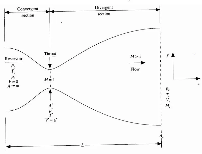
The schematic for the subsonic-supersonic isentropic nozzle flow
The governing equations (Non dimensional form)
Non-conservative form
Continuity equation: `(delrho')/(delt')=rho'(delV')/(delx')-rho'V'(del(lnA'))/(delx')-V'(delrho')/(delx')`
Momentum equation: `(delV')/(delt')=V'(delV')/(delx')-1/gamma((delT')/(delx')+(T')/(rho')(delrho')/(delx'))`
Energy equation: `(delT')/(delt')=V'(delT')/(delx')-(gamma-1)T'((delV')/(delx')+V'(del(lnA'))/(delx'))`
Conservative form
Continuity equation: `(del(rho'A'))/(delt')+(del(rho'A'V'))/(delx')=0`
Momentum equation: `(del(rho'A'V'))/(delt')+(del(rho'A'(V')^2+1/gammarho'A'))/(delx')=1/gammarho'(delA')/(delx')`
Energy equation: `(del(rho'((T')/(gamma-1)+gamma/2(V')^2)A'))/(delt')+(del(rho'((T')/(gamma-1)+gamma/2(V')^2)V'A'+rho'A'V'))/(delx')=0`
Non Dimensional quantities
Temperatue: `T'=T/T_0` Where `T_0` is temperature at inlet
Density: `rho'=rho/rho_0` Where `rho_0` is density at inlet
Distance: `x'=x/L` Where L is the length of the nozzle
Velocity: `V'=V/a_0` Where `a_0` is the speed of sound
Time: `t'=t/(L/(a_0))` Where `L/(a_0)` is characterstic time scale
Area: `A'=A/A^**` Where `A^**` is area at throat
For calculating the time step this formula is used and the minimum value is taken
`triangle t=(C*dx)/(a+v)`
Where C is Courant number
dx is grid size
a is speed of sound at that point
Main Code:
clear all
close all
clc
%GRID SIZE
n=31;
x=linspace(0,3,n);
dx=x(2)-x(1);

%VALUES FOR GAMMA, TIME STEPS,AND CFL NUMBER
gamma=1.4;
nt=1:1000;
c=0.5;

%NON-CONSERVATIVE FUNCTION CALLING
[m_dot,pressure,mach_no,rho_nc,T_nc]=non_conservative(n,x,dx,c,nt,gamma);
%CONSERVATIVE FUNCTION CALLING
[m_dot_c,pressure_c,mach_no_c,rho,T]=conservative(n,x,dx,c,gamma,nt);

%PLOT FOR COMPARSION OF MASS FLOW RATES IN BOTH FORMS
figure(7)
plot(x,m_dot_c,x,m_dot)
xlabel('Length of nozzle')
ylabel('Mass flow rate')
legend('Conservative','Non-conservative')
title('Comparison of Normalized mass flow rate distributions of both forms')
Non-conservative Function
function [m_dot,pressure,mach_no,rho_nc,T_nc]=non_conservative(n,x,dx,c,nt,gamma)

%INITIAL CONDITIONS
rho_nc=1-0.3146*x;
T_nc=1-0.2341*x;
v=(0.1+1.09*x).*T_nc.^0.5;
A=1+2.2*(x-1.5).^2;

%TO FIND DT(TIME STEP)
dt=min(c.*dx./(sqrt(T_nc)+v));

%TIME LOOP
for k=1:length(nt)
    %COPY OF VARIABLES
    rho_old=rho_nc;
    T_old=T_nc;
    v_old=v;
    %PREDICTOR LOOP
    for j=2:n-1
        drho_dx=(rho_nc(j+1)-rho_nc(j))/dx;
        dT_dx=(T_nc(j+1)-T_nc(j))/dx;
        dv_dx=(v(j+1)-v(j))/dx;
        dloga_dx=(log(A(j+1))-log(A(j)))/dx;

        %CONTINUITY EQUATION
        drho_dt_p(j)=-rho_nc(j)*dv_dx-rho_nc(j)*v(j)*dloga_dx-v(j)*drho_dx;
        %MOMENTUM EQUATION
        dv_dt_p(j)=-v(j)*dv_dx-(1/gamma)*(dT_dx+(T_nc(j)*drho_dx/rho_nc(j)));
        %ENERGY EQUATION
        dT_dt_p(j)=-v(j)*dT_dx-(gamma-1)*T_nc(j)*(dv_dx+v(j)*dloga_dx);

        %SOLUTION UPDATE
        rho_nc(j)=rho_nc(j)+drho_dt_p(j)*dt;
        T_nc(j)=T_nc(j)+dT_dt_p(j)*dt;
        v(j)=v(j)+dv_dt_p(j)*dt;
    end
    %CORRECTOR LOOP
    for j=2:n-1
        drho_dx=(rho_nc(j)-rho_nc(j-1))/dx;
        dT_dx=(T_nc(j)-T_nc(j-1))/dx;
        dv_dx=(v(j)-v(j-1))/dx;
        dloga_dx=(log(A(j))-log(A(j-1)))/dx;

        %CONTINUITY EQUATION
        drho_dt_c(j)=-rho_nc(j)*dv_dx-rho_nc(j)*v(j)*dloga_dx-v(j)*drho_dx;
        %MOMENTUM EQUATION
        dv_dt_c(j)=-v(j)*dv_dx-(1/gamma)*(dT_dx+(T_nc(j)*drho_dx/rho_nc(j)));
        %ENERGY EQUATION
        dT_dt_c(j)=-v(j)*dT_dx-(gamma-1)*T_nc(j)*(dv_dx+v(j)*dloga_dx);
    end
    %TO FIND THE AVERAGE VALUES
    drho_dt=0.5.*(drho_dt_p+drho_dt_c);
    dT_dt=0.5.*(dT_dt_p+dT_dt_c);
    dv_dt=0.5.*(dv_dt_p+dv_dt_c);

    %FINAL SOLUTION UPDATE
    for j=2:n-1
        rho_nc(j)=rho_old(j)+drho_dt(j)*dt;
        T_nc(j)=T_old(j)+dT_dt(j)*dt;
        v(j)=v_old(j)+dv_dt(j)*dt;
    end

    %BOUNDARY CONDITIONS
    %AT INFLOW
    rho_nc(1)=1;
    v(1)=2*v(2)-v(3);
    T_nc(1)=1;
    %AT OUTFLOW
    rho_nc(n)=2*rho_nc(n-1)-rho_nc(n-2);
    T_nc(n)=2*T_nc(n-1)-T_nc(n-2);
    v(n)=2*v(n-1)-v(n-2);

    %CALCULATING MASS FLOW RATE, PRESSURE AND MACH NUMBER
    m_dot=rho_nc.*A.*v;
    pressure=rho_nc.*T_nc;
    mach_no=v./sqrt(T_nc);

    %CALCULATING VALUES AT THROAT SECTION
    rho_throat(k)=rho_nc(16);
    T_throat(k)=T_nc(16);
    v_throat(k)=v(16);
    m_dot_throat(k)=m_dot(16);
    pressure_throat(k)=pressure(16);
    mach_no_throat(k)=mach_no(16);

    %PLOT FOR MASS FLOW RATE AT DIFF TIME STEPS
    figure(1)
    if k==1
        plot(x,m_dot)
        hold on
    elseif k==50
        plot(x,m_dot)
        hold on
    elseif k==100
        plot(x,m_dot)
        hold on
    elseif k==150
        plot(x,m_dot)
        hold on
    elseif k==200
        plot(x,m_dot)
        hold on
    elseif k==700
        plot(x,m_dot)
        hold on
    elseif k==1000
        plot(x,m_dot)
        hold on
    end
    title('Variation of Mass flow rate inside the nozzle at different time steps')
    xlabel('distance')
    ylabel('mass flow rate')
    legend('@ 1','@ 50','@ 150','@ 200','@ 700','@ 1000')
end
%PLOT OF PRIMITVE VARIABLES AFTER STEADY STATE
figure(2)
plot(x,v,x,T,x,rho,x,mach_no,x,pressure,x,m_dot)
title('Steady-state distribution of primitive variables inside the nozzle')
xlabel('distance')
ylabel('Non dimensional variables')
legend('Velocity','Temperature','Density','Mach number','Pressure','Mass flow rate')

%PLOT OF TIME VARIATION OF PRIMITIVE VARIABLES
figure(3)
plot(nt,rho_throat,nt,T_throat,nt,v_throat,nt,pressure_throat,nt,m_dot_throat,nt,mach_no_throat)
title('Time-wise variation of the primitive variables')
xlabel('Time steps')
ylabel('Non dimensional variables')
legend('Density','Temperature','Velocity','Pressure','Mass flow rate','Mach number')
end
Conservative function
function [m_dot_c,pressure_c,mach_no_c,rho,T]=conservative(n,x,dx,c,gamma,nt)
%INITIAL CONDITIONS
for i=1:n
    if (x(i)>=0 && x(i)<=0.5)
        rho(i)=1;
        T(i)=1;
    elseif (x(i)>=0.5 && x(i)<=1.5)
        rho(i)=1-0.366*(x(i)-0.5);
        T(i)=1-0.167*(x(i)-0.5);
    elseif (x(i)>=1.5 && x(i)<=3)
        rho(i)=0.634-0.3879*(x(i)-1.5);
        T(i)=0.833-0.3507*(x(i)-1.5);
    end
end
A=1+2.2*(x-1.5).^2;
v=0.59./(rho.*A);
pressure_c=rho.*T;

%DEFINING SOLUTION VECTORS
u1=rho.*A;
u2=rho.*A.*v;
u3=rho.*A.*(T./(gamma-1)+(gamma/2).*v.^2);

%TO CALCULATE TIME STEP
dt=min(c.*dx./(sqrt(T)+v));

%TIME LOOP
for k=1:length(nt)
    %COPY OF VARIABLES
    u1_old=u1;
    u2_old=u2;
    u3_old=u3;

    %DEFINING FLUX VECTORS
    f1=u2;
    f2=((u2.^2)./u1)+((gamma-1)/gamma)*(u3-(gamma/2)*((u2.^2)./u1));
    f3=((gamma*u2.*u3)./u1)-(gamma*(gamma-1)*((u2.^3)./(2*u1.^2)));

    %PREDICTOR LOOP
    for j=2:n-1

        %DEFINING SOURCE TERM
        J(j)=(1/gamma)*rho(j)*T(j)*((A(j+1)-A(j))/dx);

        %CONTINUITY EQUATION
        du1_dt_p(j)=-((f1(j+1)-f1(j))/dx);
        %MOMENTUM EQUATION
        du2_dt_p(j)=-((f2(j+1)-f2(j))/dx)+J(j);
        %ENERGY EQUATION
        du3_dt_p(j)=-((f3(j+1)-f3(j))/dx);

        %SOLUTION UPDATE
        u1(j)=u1(j)+du1_dt_p(j)*dt;
        u2(j)=u2(j)+du2_dt_p(j)*dt;
        u3(j)=u3(j)+du3_dt_p(j)*dt;
    end

    %UPDATING FLUX TERMS
    f1=u2;
    f2=((u2.^2)./u1)+((gamma-1)/gamma)*(u3-(gamma/2)*((u2.^2)./u1));
    f3=((gamma*u2.*u3)./u1)-(gamma*(gamma-1)*((u2.^3)./(2*u1.^2)));

    %CORRECTOR LOOP
    for j=2:n-1

        %DEFINING SOURCE TERM
        J(j)=(1/gamma)*rho(j)*T(j)*((A(j)-A(j-1))/dx);
        %CONTINUITY EQUATION
        du1_dt_c(j)=-(f1(j)-f1(j-1))/dx;
        %MOMENTUM EQUATION
        du2_dt_c(j)=-(f2(j)-f2(j-1))/dx+J(j);
        %ENERGY EQUATION
        du3_dt_c(j)=-(f3(j)-f3(j-1))/dx;
    end

    %TO CALCULATE AVERAGE VALUES
    du1_dt=0.5*(du1_dt_p+du1_dt_c);
    du2_dt=0.5*(du2_dt_p+du2_dt_c);
    du3_dt=0.5*(du3_dt_p+du3_dt_c);

    %FINAL SOLUTION UPDATE
    for j=2:n-1
       u1(j)=u1_old(j)+du1_dt(j)*dt;
       u2(j)=u2_old(j)+du2_dt(j)*dt;
       u3(j)=u3_old(j)+du3_dt(j)*dt;
    end
    %INITIAL CONDITIONS
    %AT INFLOW
    u1(1)=rho(1)*A(1);
    u2(1)=2*u2(2)-u2(3);
    u3(1)=u1(1)*(T(1)/(gamma-1)+(gamma/2)*(u2(1)/u1(1))^2);
    %AT OUTFLOW
    u1(n)=2*u1(n-1)-u1(n-2);
    u2(n)=2*u2(n-1)-u2(n-2);
    u3(n)=2*u3(n-1)-u3(n-2);

    %FINDING PRIMITIVE VARIABLES FROM SOLUTION VECTORS
    rho=u1./A;
    v=u2./u1;
    T=(gamma-1)*(u3./u1-(gamma/2)*v.^2);

    %CALCULATING MASS FLOW RATE, PRESSURE AND MACH NUMBER
    m_dot_c=u2;
    pressure_c=rho.*T;
    mach_no_c=v./sqrt(T);

    %CALCULATING VALUES AT THROAT SECTION
    rho_throat(k)=rho(16);
    T_throat(k)=T(16);
    v_throat(k)=v(16);
    m_dot_throat(k)=m_dot_c(16);
    pressure_throat(k)=pressure_c(16);
    mach_no_throat(k)=mach_no_c(16);

    %PLOT FOR MASS FLOW RATE AT DIFF TIME STEPS
    figure(4)
    if k==1
        plot(x,m_dot_c)
        hold on
    elseif k==50
        plot(x,m_dot_c)
        hold on
    elseif k==100
        plot(x,m_dot_c)
        hold on
    elseif k==150
        plot(x,m_dot_c)
        hold on
    elseif k==200
        plot(x,m_dot_c)
        hold on
    elseif k==700
        plot(x,m_dot_c)
        hold on
    elseif k==1000
        plot(x,m_dot_c,'o')
        hold on
    end
    title('Variation of Mass flow rate inside the nozzle at different time steps')
    xlabel('distance')
    ylabel('mass flow rate')
    legend('@ 1','@ 50','@ 150','@ 200','@ 700','@ 1000')
end

%PLOT OF PRIMITVE VARIABLES AFTER STEADY STATE
figure(5)
plot(x,v,x,T,x,rho,x,mach_no_c,x,pressure_c,x,m_dot_c)
title('Steady-state distribution of primitive variables inside the nozzle')
xlabel('distance')
ylabel('Non dimensional variables')
legend('Velocity','Temperature','Density','Mach number','Pressure','Mass flow rate')

%PLOT OF TIME VARIATION OF PRIMITIVE VARIABLES
figure(6)
plot(nt,rho_throat,nt,T_throat,nt,v_throat,nt,pressure_throat,nt,m_dot_throat,nt,mach_no_throat)
title('Time-wise variation of the primitive variables')
xlabel('Time steps')
ylabel('Non dimensional variables')
legend('Density','Temperature','Velocity','Pressure','Mass flow rate','Mach number')
end
Results:
Non-conservative form
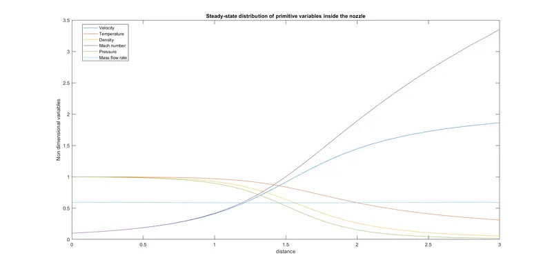
Values of primitive variables along the nozzle after reaching steady state, The values is similar to the exact solution than conservative form.
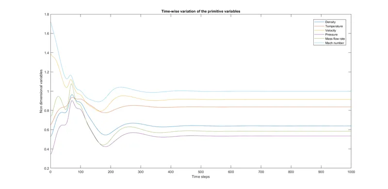
From this plot we can see that at early time steps the value of primitive variables is large and tend to oscillate and as the time step increases the values becomes small and finally reaches a constant value
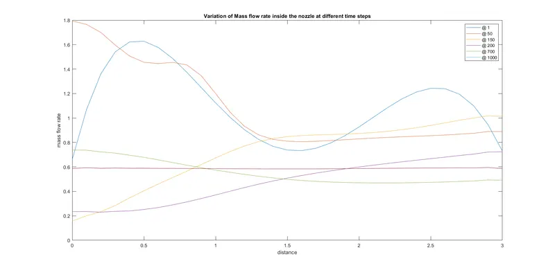
We can see that as the time step increases the mass flow rate is almost becoming constant.
Conservative form
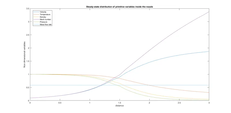
Values of primitive variables along the nozzle after reaching steady state, we can see slight variations in the curve and is not as accurate as the non-conservative form.
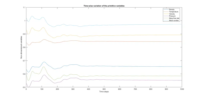
Here also we see the same pattern large and oscillating at start and becomes smaller with time and reaches constant value but in conservative form oscillation is less and hence attaining steady state faster.
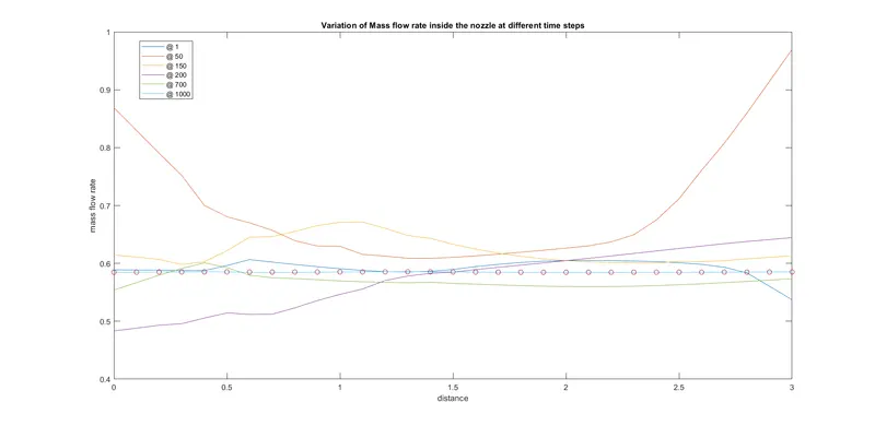
We can see that as the time step increases the mass flow rate is almost becoming constant and is also converges faster than non-conservative form
Conclusion:
Non-conservative vs Conservative form
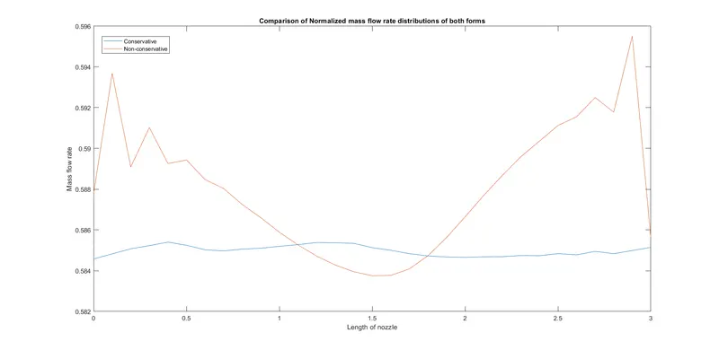
As we can see from the above plot that the conservative form has better mass flow rate distributions that the non-conservative form this can be said due to 2 major factors:
The first one being that the non-conservative form has some variations in the inflow and the outflow boundary regions where as the conservative form has almost very less variations.
The second point is that the conservative form's value is much closer to the exact solution (0.579) than the non-conservative form.
Hence it can be concluded that the conservative form is better at conserving mass than the non-conservative form.
Grid Independence test
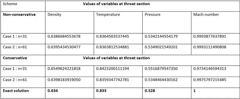
From the above table it can be seen that the values of the primitive variables at throat section for both the grid points(n=31,61) is almost similar in both the forms, Hence it can be said that the solution is Grid Independent.
If we take a closer look at the values of both the conservative and non-conservative form we can see that the non-conservative form is slightly closer to exact solution that the conservative form this is mainly because the non-conservative form leads to smaller residuals, So it can be said that the non-conservative form can give slightly accurate results compared to the conservative form.
The conservative form is also time consuming than the non-conservative forms this is mainly due to splitting of the equation into solution , flux vectors.