Week 5.1 - Mid term project - Solving the steady and unsteady 2D heat conduction problem
Aim:
To solve steady and unsteady 2-D heat conduction equation using point iterative methods
Objective:
- To solve 2-D steady state heat conduction equation using Jacobi,Gauss-Seidel,Successive over-relaxation methods
- To solve 2-D unsteady state heat conduction equation by using both explicit and implicit schemes
- To plot the temperature contour for all the methods
Assumptions:
The domain is a unit square
Number of grid points along x is equal to number of grid points along y (nx=ny)
Boundary conditions as:
Top Boundary = 600 K
Bottom Boundary = 900 K
Left Boundary = 400 K
Right Boundary = 800 K
Steady state:
Theory:
The steady state 2-D heat conduction equation is:
`(del^2t)/(delx^2)+(del^2t)/(dely^2)=0`
By discretising the above equation we get:
`T(i,j)=1/K((T_l+T_r)/(trianglex^2)+(T_t+T_b)/(triangley^2))`
Where
`K=2*((trianglex^2+triangley^2)/(trianglex^2*triangley^2))`
`T_l=` Temperatue to the left of current point
`T_r=` Temperatue to the right of current point
`T_t=` Temperatue to the top of current point
`T_b=` Temperatue to the bottom of current point
Code:
clear all
close all
clc

%GRID SIZE
nx=10;
ny=nx;
x=linspace(0,1,nx);
y=linspace(0,1,ny);
dx=x(2)-x(1);
dy=y(2)-y(1);

%GIVEN INPUTS
error=9e9;           %ERROR CAN BE ANY VALUE GREATER THAN TOLERANCE
tolerance=1e-4;
t_left=400;
t_right=800;
t_top=600;
t_bot=900;

%iNITIALIZING THE BOUNDARY CONDITIONS
t=300*ones(nx,ny);
t(2:ny-1,1)=t_left;
t(2:ny-1,nx)=t_right;
t(1,2:nx-1)=t_top;
t(ny,2:nx-1)=t_bot;
%ASSIGNING VALUES AT THR CORNERS
t(1,1)=(t_top+t_left)/2;
t(1,nx)=(t_top+t_right)/2;
t(ny,nx)=(t_bot+t_right)/2;
t(ny,1)=(t_bot+t_left)/2;

t_old=t;
k=2*((dx^2+dy^2)/(dx^2*dy^2));

%VARIABLE TO CHANGE THE ITERATIVE METHOD
iterative_solver=3;

%JACOBI METHOD
if iterative_solver==1
    j_iteration=1;
    %CONVERGENCE LOOP
    while(error>tolerance)
        %SPACE LOOP
        for i=2:ny-1
            for j=2:nx-1
                term1=(t_old(i-1,j)+t_old(i+1,j))/(k*dx^2);
                term2=(t_old(i,j+1)+t_old(i,j-1))/(k*dy^2);
                t(i,j)=term1+term2;
            end
        end
        %UPDATE ERROR AND TEMPERATURE AND CALCULATE THE NUMBER OF ITERATIONS
        error=max(max(abs(t_old-t)));
        t_old=t;
        j_iteration=j_iteration+1;
    end
%PLOTING THE TEMPERATURE CONTOUR
figure(1)
contourf(x,y,t)
clabel(contourf(x,y,t))
colorbar
colormap(jet)
set(gca,'ydir','reverse')
xlabel('X AXIS')
ylabel('Y AXIS')
title(sprintf('no of jacobi iterations=%d',j_iteration));
pause(0.3)
end
%GAUSS-SEIDEL METHOD
if iterative_solver==2
    gs_iteration=1;
    %CONVERGENCE LOOP
    while(error>tolerance)
         %SPACE LOOP
        for i=2:ny-1
            for j=2:nx-1
                term1=(t(i-1,j)+t_old(i+1,j))/(k*dx^2);
                term2=(t_old(i,j+1)+t(i,j-1))/(k*dy^2);
                t(i,j)=term1+term2;
            end
        end
        %UPDATE ERROR AND TEMPERATURE AND CALCULATE THE NUMBER OF ITERATIONS
        error=max(max(abs(t_old-t)));
        t_old=t;
        gs_iteration=gs_iteration+1;
    end
%PLOTING THE TEMPERATURE CONTOUR
figure(2)
contourf(x,y,t)
clabel(contourf(x,y,t))
colorbar
colormap(jet)
set(gca,'ydir','reverse')
xlabel('X AXIS')
ylabel('Y AXIS')
title(sprintf('no of gauss siedel iterations=%d',gs_iteration));
pause(0.3)
end
%SOR METHOD
if iterative_solver==3
    sor_iteration=1;
    omega=1.5;
    %CONVERGENCE LOOP
    while(error>tolerance)
        %SPACE LOOP
        for i=2:ny-1
            for j=2:nx-1
                t(i,j)=omega*((t(i-1,j)+t_old(i+1,j))/(k*dx^2)+(t_old(i,j+1)+t(i,j-1))/(k*dy^2))+(1-omega)*t_old(i,j);
            end
        end
         %UPDATE ERROR AND TEMPERATURE AND CALCULATE THE NUMBER OF ITERATIONS
        error=max(max(abs(t_old-t)));
        t_old=t;
        sor_iteration=sor_iteration+1;
    end
%PLOTING THE TEMPERATURE CONTOUR
figure(3)
contourf(x,y,t)
clabel(contourf(x,y,t))
colorbar
colormap(jet)
set(gca,'ydir','reverse')
xlabel('X AXIS')
ylabel('Y AXIS')
title(sprintf('no of gauss siedel iterations=%d',sor_iteration));
pause(0.3)
end
Output:
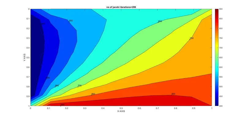
Jacobi
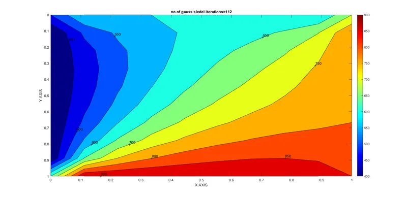
Gauss_seidel
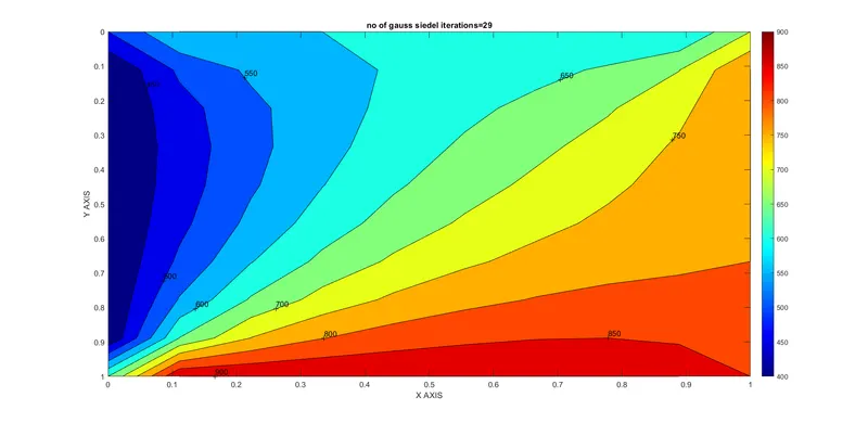
Successive over-relaxation
Unsteady state:
- Explicit scheme:
Theory:
The unsteady state 2-D heat conduction equation is:
`(delT)/(delt)=alpha*((del^2t)/(delx^2)+(del^2t)/(dely^2))`
By discretising the above equation we get:
`(T_p^(n+1)-T_p^n)/(trianglet)=alpha((T_l-2T_p+T_r)/(trianglex^2)+(T_t-2T_p+T_b)/(triangley^2))`
further simplfying we get:
`T_p^(n+1)=(1/(1+2K_1+2K_2))*[T_p^n+K_1(T_l+T_r)^n+K_2(T_t+T_b)^n]`
Where
`K_1=(alphatrianglet)/(trianglex^2)`
`K_2=(alphatrianglet)/(triangley^2)`
`T_l=` Temperatue to the left of current point
`T_r=` Temperatue to the right of current point
`T_t=` Temperatue to the top of current point
`T_b=` Temperatue to the bottom of current point
Code:
clear all
close all
clc

%GRID SIZE AND TIME STEP
nx=10;
ny=nx;
dt=0.001;
x=linspace(0,1,nx);
y=linspace(0,1,ny);
dx=x(2)-x(1);
dy=y(2)-y(1);

%THERMAL DIFFUSIVITY
alpha=1.4;

%GIVEN INPUTS
error=9e9;           %ERROR CAN BE ANY VALUE GREATER THAN TOLERANCE
tolerance=1e-4;
t_left=400;
t_right=800;
t_top=600;
t_bot=900;

%iNITIALIZING THE BOUNDARY CONDITIONS
t=300*ones(nx,ny);
t(2:ny-1,1)=t_left;
t(2:ny-1,nx)=t_right;
t(1,2:nx-1)=t_top;
t(ny,2:nx-1)=t_bot;
%ASSIGNING VALUES AT THR CORNERS
t(1,1)=(t_top+t_left)/2;
t(1,nx)=(t_top+t_right)/2;
t(ny,nx)=(t_bot+t_right)/2;
t(ny,1)=(t_bot+t_left)/2;

t_old=t;
k1=alpha*(dt/(dx^2));
k2=alpha*(dt/(dy^2));
iteration=1;
%TIME LOOP
for nt=1:1400
    %SPACE LOOP
    for i=2:ny-1
        for j=2:nx-1
            t(i,j)=t_old(i,j)+k1*(t_old(i-1,j)-2*t_old(i,j)+t_old(i+1,j))+k2*(t_old(i,j-1)-2*t_old(i,j)+t_old(i,j+1));
        end
    end
    %UPDATE TEMPERATURE AND CALCULATE THE NUMBER OF ITERATIONS
    iteration=iteration+1;
    t_old=t;
end
%PLOTING THE TEMPERATURE CONTOUR
figure(1)
contourf(x,y,t)
clabel(contourf(x,y,t))
colorbar
colormap(jet)
set(gca,'ydir','reverse')
xlabel('X AXIS')
ylabel('Y AXIS')
title(sprintf('no of iterations=%d',iteration));
pause(0.3)
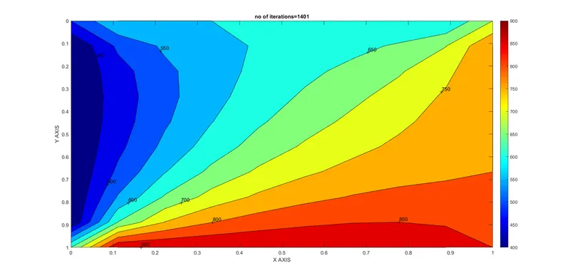
Output:
2. Implicit scheme:
Theory:
The unsteady state 2-D heat conduction equation is:
`(delT)/(delt)=alpha*((del^2t)/(delx^2)+(del^2t)/(dely^2))`
By discretising the above equation we get:
`(T_p^(n+1)-T_p^n)/(trianglet)=alpha((T_l-2T_p+T_r)/(trianglex^2)+(T_t-2T_p+T_b)/(triangley^2))`
further simplfying we get:
`T_p^(n+1)=(1/(1+2K_1+2K_2))*[T_p^n+K_1(T_l+T_r)^(n+1)+K_2(T_t+T_b)^(n+1)]`
Where
`K_1=(alphatrianglet)/(trianglex^2)`
`K_2=(alphatrianglet)/(triangley^2)`
`T_l=` Temperatue to the left of current point
`T_r=` Temperatue to the right of current point
`T_t=` Temperatue to the top of current point
`T_b=` Temperatue to the bottom of current point
Code:
clear all
close all
clc

%GRID SIZE AND TIME STEP
nx=10;
ny=nx;
dt=0.001;
x=linspace(0,1,nx);
y=linspace(0,1,ny);
dx=x(2)-x(1);
dy=y(2)-y(1);

%THERMAL DIFFUSIVITY
alpha=1.4;

omega=1.1;

%GIVEN INPUTS
tolerance=1e-4;
t_left=400;
t_right=800;
t_top=600;
t_bot=900;

%iNITIALIZING THE BOUNDARY CONDITIONS
t=300*ones(nx,ny);
t(2:ny-1,1)=t_left;
t(2:ny-1,nx)=t_right;
t(1,2:nx-1)=t_top;
t(ny,2:nx-1)=t_bot;
%ASSIGNING VALUES AT THE CORNERS
t(1,1)=(t_top+t_left)/2;
t(1,nx)=(t_top+t_right)/2;
t(ny,nx)=(t_bot+t_right)/2;
t(ny,1)=(t_bot+t_left)/2;

%VARIABLES FOR TIME LOOP AND SPACE LOOP
t_old=t;
t_prev=t;

k1=alpha*(dt/(dx^2));
k2=alpha*(dt/(dy^2));

%VARIABLE TO CHANGE THE ITERATIVE METHOD
iterative_solver=3;

%JACOBI METHOD
if iterative_solver==1
    j_iteration=1;
    %TIME LOOP
    for nt=1:1400
        error=9e9; %ERROR CAN BE ANY VALUE GREATER THAN TOLERANCE
        %CONVERGENCE LOOP
        while(error>tolerance)
            %SPACE LOOP
            for i=2:ny-1
                for j=2:nx-1
                    term1=(1+2*k1+2*k2)^-1;
                    term2=k1*term1;
                    term3=k2*term1;
                    H=(t_old(i-1,j)+t_old(i+1,j));
                    V=(t_old(i,j-1)+t_old(i,j+1));
                    t(i,j)=((t_prev(i,j)*term1)+(H*term2)+(V*term3));
                end
            end
            %UPDATE ERROR AND TEMPERATURE AND CALCULATE THE NUMBER OF ITERATIONS
            error=max(max(abs(t_old-t)));
            t_old=t;
            j_iteration=j_iteration+1;
        end
        t_prev=t;
    end
    %PLOTING THE TEMPERATURE CONTOUR
    figure(1)
    contourf(x,y,t)
    clabel(contourf(x,y,t))
    colorbar
    colormap(jet)
    set(gca,'ydir','reverse')
    xlabel('X AXIS')
    ylabel('Y AXIS')
    title(sprintf('no of Transient jacobi iterations=%d',j_iteration));
end

%GAUSS-SEIDEL METHOD
if iterative_solver==2
    gs_iteration=1;
    %TIME LOOP
    for nt=1:1400
        error=9e9; %ERROR CAN BE ANY VALUE GREATER THAN TOLERANCE
        %CONVERGENCE LOOP
        while(error>tolerance)
            %SPACE LOOP
            for i=2:ny-1
                for j=2:nx-1
                    term1=(1+2*k1+2*k2)^-1;
                    term2=k1*term1;
                    term3=k2*term1;
                    H=(t(i-1,j)+t_old(i+1,j));
                    V=(t(i,j-1)+t_old(i,j+1));
                    t(i,j)=((t_prev(i,j)*term1)+(H*term2)+(V*term3));
                end
            end
            %UPDATE ERROR AND TEMPERATURE AND CALCULATE THE NUMBER OF ITERATIONS
            error=max(max(abs(t_old-t)));
            t_old=t;
            gs_iteration=gs_iteration+1;
        end
        t_prev=t;
    end
    %PLOTING THE TEMPERATURE CONTOUR
    figure(2)
    contourf(x,y,t)
    clabel(contourf(x,y,t))
    colorbar
    colormap(jet)
    set(gca,'ydir','reverse')
    xlabel('X AXIS')
    ylabel('Y AXIS')
    title(sprintf('no of Transient Gauss-seidel iterations=%d',gs_iteration));
end

%SUCCESSIVE OVER-RELAXATION METHOD
if iterative_solver==3
    sor_iteration=1;
    %TIME LOOP
    for nt=1:1400
        error=9e9; %ERROR CAN BE ANY VALUE GREATER THAN TOLERANCE
        %CONVERGENCE LOOP
        while(error>tolerance)
            %SPACE LOOP
            for i=2:ny-1
                for j=2:nx-1
                    term1=(1+2*k1+2*k2)^-1;
                    term2=k1*term1;
                    term3=k2*term1;
                    H=(t(i-1,j)+t_old(i+1,j));
                    V=(t(i,j-1)+t_old(i,j+1));
                    t(i,j)=omega*(((t_prev(i,j)*term1)+(H*term2)+(V*term3)))+((1-omega)*t_old(i,j));
                end
            end
            %UPDATE ERROR AND TEMPERATURE AND CALCULATE THE NUMBER OF ITERATIONS
            error=max(max(abs(t_old-t)));
            t_old=t;
            sor_iteration=sor_iteration+1;
        end
        t_prev=t;
    end
    %PLOTING THE TEMPERATURE CONTOUR
    figure(3)
    contourf(x,y,t)
    clabel(contourf(x,y,t))
    colorbar
    colormap(jet)
    set(gca,'ydir','reverse')
    xlabel('X AXIS')
    ylabel('Y AXIS')
    title(sprintf('no of Transient SOR iterations=%d',sor_iteration));
end
Output:
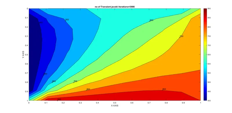
Jacobi:
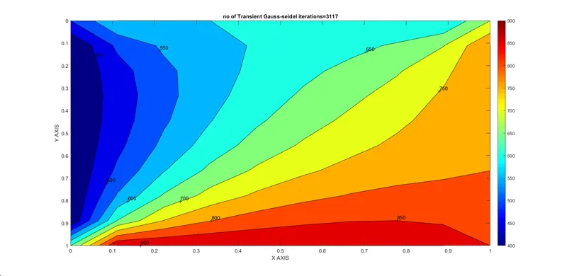
Gauss-seidel:
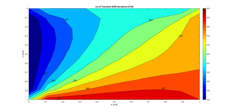
Successive over-relaxation:
Conclusion:
For the given grid size(nx=ny=10),time size(dt=0.001) and total time steps(nt=1400) the number of iterations for various methods are:
| Type of analysis | Jacobi Iterations | Gauss-seidel Iterations | Successive over-relaxation iterations |
| Steady state | 208 | 112 | 29 |
| Transient - Implicit | 3666 | 3117 | 2745 |
Transient- Explicit -1401
From the above table we can see that the Jacobi iterations are greater than Gauss-seidel and Successive over-relaxation having the least number of iterations , hence it can be said that Successive over-relaxation method is more efficient iterative methods than Gauss-seidel and Jacobi if the value for the over-relaxation coefficent(omega) is given properly.
For the steady state analysis the value of omega was 1.5 and for the Transient implicit analysis the omega value was 1.1, If this values are further increased the number of iterations also increases due to oscilation of the solution.
The steady state analysis takes very less iterations since there is no time variable and hence avoiding the time loop.
We can also see that the explicit method does not require any point iterative methods because in each equation all the values are known and hence can be calculated at that point without any numerical methods.