Deriving 4th order approximation of a 2nd order derivative

QUESTION:

Derive the following 4th order approximations of the second-order derivative.

1. Central difference
2. Skewed right-sided difference
3. Skewed left-sided difference

After deriving these schemes, prove that your skewed schemes are fourth-order accurate.

Once you have done this, write a program in MATLAB to evaluate the second-order derivative of the analytical function exp(x)*cos(x) and compare it with the 3 numerical approximations that you have derived.

Provide a plot that compares the absolute error between the above-mentioned schemes

In your own words, describe why a skewed scheme is useful? What can a skewed scheme do that a CD scheme cannot?

ANSWER:

TAYLOR SERIES:

• The Taylor series of a function is an infinite sum of terms that are expressed in terms of the function derivative at a single point.
• For the most common function, the function and the sum of its Taylor series are equal near this point.

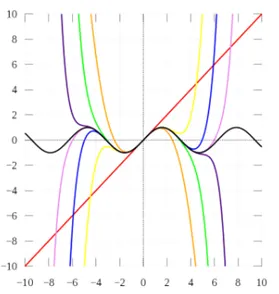
• As the degree of the Taylor polynomial rises, it approaches the correct function. This image shows sin x and its Taylor approximation by a polynomial of degree 1,3, 5, 7, 9, 11, and 13 at x = 0

INPUT: -

[MATLAB CODE]

%% Initialization
clc
clear all
close all

%% Values of X and Dx

x = pi/3;
dx = linspace(pi/4,pi/400,200);

%% Given Function

% function = exp(x)*cos(x)
% Analytical Value = -2*exp(x)*sin(x)

Analytical_Derivative = -2*exp(x)*sin(x);


%% Left side skewed 

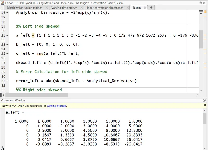
a_left = [1 1 1 1 1 1 ; 0 -1 -2 -3 -4 -5 ; 0 1/2 4/2 9/2 16/2 25/2 ; 0 -1/6 -8/6 -27/6 -64/6 -125/6 ; 0 1/24 16/24 81/24 256/24 625/24 ; 0 -1/120 -32/120 -243/120 -1024/120 -3125/120];

b_left = [0; 0; 1; 0; 0; 0];

c_left = inv(a_left)*b_left;

skewed_left = (c_left(1).*exp(x).*cos(x)+c_left(2).*exp(x-dx).*cos(x-dx)+c_left(3).*exp(x-2.*dx).*cos(x-2.*dx)+c_left(4).*exp(x-3.*dx).*cos(x-3.*dx)+c_left(5).*exp(x-4.*dx).*cos(x-4.*dx)+c_left(6).*exp(x-5.*dx).*cos(x-5.*dx))./(dx.^2);

% Error Calculation for left side skewed

error_left = abs(skewed_left - Analytical_Derivative);

%% Right side skewed 

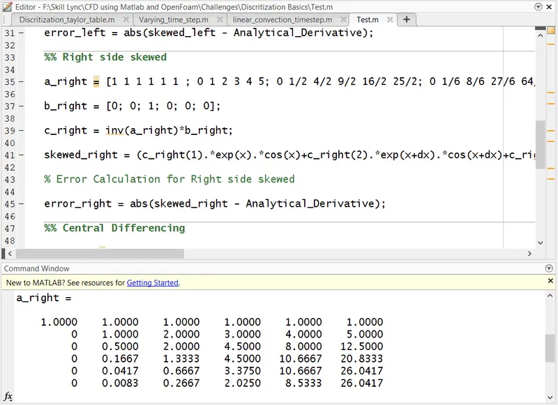
a_right = [1 1 1 1 1 1 ; 0 1 2 3 4 5; 0 1/2 4/2 9/2 16/2 25/2; 0 1/6 8/6 27/6 64/6 125/6 ; 0 1/24 16/24 81/24 256/24 625/24 ; 0 1/120 32/120 243/120 1024/120 3125/120];

b_right = [0; 0; 1; 0; 0; 0];

c_right = inv(a_right)*b_right;

skewed_right = (c_right(1).*exp(x).*cos(x)+c_right(2).*exp(x+dx).*cos(x+dx)+c_right(3).*exp(x+2.*dx).*cos(x+2.*dx)+c_right(4).*exp(x+3.*dx).*cos(x+3.*dx)+c_right(5).*exp(x+4.*dx).*cos(x+4.*dx)+c_right(6).*exp(x+5.*dx).*cos(x+5.*dx))./(dx.^2);

% Error Calculation for Right side skewed

error_right = abs(skewed_right - Analytical_Derivative);

%% Central Differencing

a_centre = [1 1 1 1 1; -2 -1 0 1 2; 4/2 1/2 0 1/2 4/2; -8/6 -1/6 0 1/6 8/6; 16/24 1/24 0 1/24 16/24];

b_centre = [0; 0; 1; 0; 0];

c_centre = inv(a_centre)*b_centre;

centre_difference = (c_centre(1).*exp(x-2.*dx).*cos(x-2.*dx)+c_centre(2).*exp(x-dx).*cos(x-dx)+c_centre(3).*exp(x).*cos(x)+c_centre(4).*exp(x+dx).*cos(x+dx)+c_centre(5).*exp(x+2.*dx).*cos(x+2.*dx))./((dx).^2);

% Error calculation for center differencing

error_centre = abs(centre_difference - Analytical_Derivative);

%% Plotting


loglog(dx,error_left,'linewidth',2);
hold on
loglog(dx,error_right,'linewidth',2);
loglog(dx,error_centre,'linewidth',2);
grid on
xlabel('dx');
ylabel('Error');
legend('Skewed Left-Side','Skewed Right-Side','Central Differencing')

EXPLANATION: -

• Value of x is taken as
• Defining the step size, dx = linspace(pi/4,pi/400,200)
• Analytical function - exp(x)*cos(x)
• The analytical second-order derivative function is expressed as

• For the left, right, and central differencing the constants are calculated for A, X, and B values.

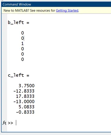
Coefficients for Left Side Skewed Differencing:

• The following coefficients for left-skewed are calculated from MATLAB code:

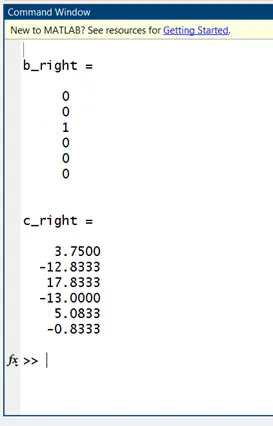
Coefficients for Right Side Skewed Differencing:

• The following coefficients for right-skewed are calculated from MATLAB code:

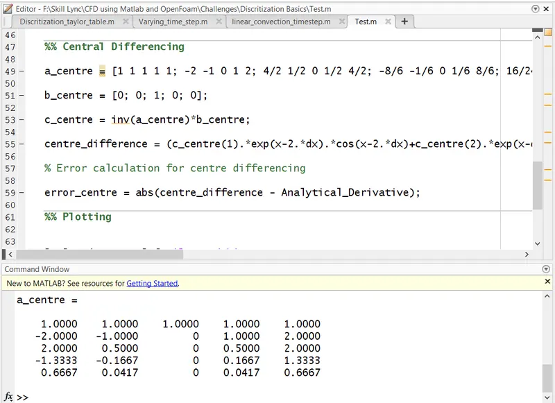
Coefficients for Central Differencing:

The following coefficients for central differencing are calculated from MATLAB code:

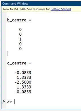
• For calculating the error for all the three differencing schemes following expression is implemented.

error_left = abs(skewed_left - Analytical_Derivative);

error_right = abs(skewed_right - Analytical_Derivative);

error_centre = abs(centre_difference - Analytical_Derivative);

• Here, by the use of ‘absolute’ command which is inbuilt MATLAB command the error is calculated.
• Next the ‘plot’ command is used for plotting the graph in between the errors with respect to grid spacing.

PLOT:

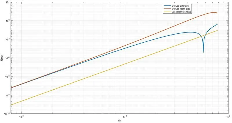
• From the above figure, we can conclude that the error for the central difference method is much lesser than the right and left-skewed methods.
• The right and Left skewed difference methods almost give the same results in terms of error for a small value of time step.

In your own words, describe why a skewed scheme is useful? What can a skewed scheme do that a CD scheme cannot?

ANSWER:

• When data from the grid point is only available from either the left or right end i.e., at node closer from the boundaries, for computation that requires the higher-order approximation we make use of the skewed scheme.
• Having a symmetric stencil is not possible for such a case hence central differencing scheme is cannot be applied.
• A skewed scheme is useful when we have data at the boundaries of our domain.
• Predicting the data from central differencing is not possible. Hence, a skewed scheme plays a very important role in such a case.

CONCLUSION:

• Hence the 4th order approximations of the second-order derivative are been explained and performed for left-skewed, right-skewed, and central differencing using the Taylor table method.
• Error for left, right, and central differencing have been compared by plotting the errors with respect to the grid spacing.
• Why a skewed scheme is useful and what a skewed scheme can do that a central scheme cannot is been explained clearly.