Week 3.5 - Deriving 4th order approximation of a 2nd order derivative using Taylor Table method

OBJECTIVE:

Fourth-order approximation for different solving methods and to prove the skewed method of solving is more accurate by giving appropriate plots and results.

GIVEN:

P : The order of accuracy

N : Number of nodes in stencil

Q : Order of derivative

SCHEME DERIVATIONS:

Nodes are classified as P + Q, so the number of nodes is 6.

Right Sided:

Equation:

∂²u/∂x² = [af(i) + bf(i+1) + cf(i+2) + df(i+3) + ef(i+4) + gf(i+5).......]/dx²

From the Taylor series of expansion in the Taylor table method,

dx2 f'' (i)	f (i)	f' (i) dx	f'' (i) dx2	f''' (i) dx3	f'''' (i) dx4	f''''' (i) dx5
af(i)	a	0	0	0	0	0
bf(i+1)	b	b	b/2	b/6	b/24	b/120
cf(i+2)	c	2c	4c/2	8c/6	16c/24	32c/120
df(i+3)	d	3d	9d/2	27d/6	81d/24	243d/120
ef(i+4)	e	4e	16e/2	64e/6	256e/24	1024e/120
gf(i+5)	g	5g	25g/2	125g/6	625g/24	3125g/120
Sum of co-efficients	0	0	1	0	0	0

In matrix form,

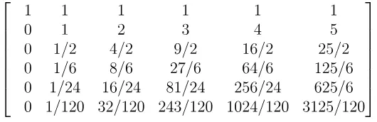
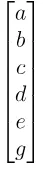
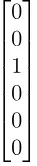
AX = B

X = inv (A) * B

From Matlab,

A = [1 1 1 1 1 1;
    0 1 2 3 4 5;
    0 1/2 4/2 9/2 16/2 25/2;
    0 1/6 8/6 27/6 64/6 125/6;
    0 1/24 16/24 81/24 256/24 625/24;
    0 1/120 32/120 243/120 1024/120 3125/120;];
B = [0;
    0;
    1;
    0;
    0;
    0;];
y = inv(A);
X = y * B

Fig:

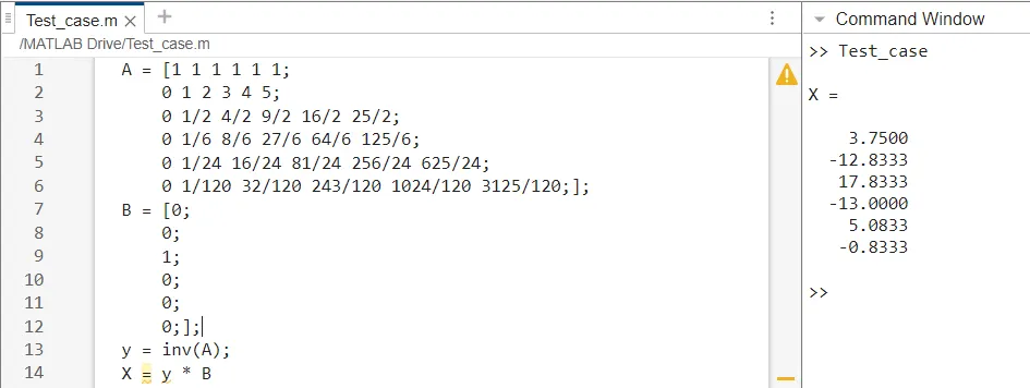
Here, X Stands for unknowns. By equating them,

a = 3.7500

b = -12.8333

c = 17.8333

d = -13.0000

e = 5.0833

g = -0.8333

Substituting these equations,

∂²u/∂x² = [(3.75) f (i) + (-12.8333) f (i + 1) + (17.8333) f (i + 2) + (-13) f (i + 3) + (5.0833) f (i + 4) + (-0.8333) f (i + 5)]/dx²

----XXXX----XXXX----XXXX----XXXX----

LEFT-SIDED:

EQUATION:

∂²u/∂x² = [af(i-5) + bf(i-4) + cf(i-3) + df(i-2) + ef(i-1) + gf(i).......]/dx²

From Taylor's series,

dx2 f'' (i)	f (i)	f' (i) dx	f'' (i) dx2	f''' (i) dx3	f'''' (i) dx4	f''''' (i) dx5
af(i-5)	a	-5a	25a/2	-125a/6	625a/24	-3125a/120
bf(i-4)	b	-4b	16b/2	-64b/6	256b/24	-1024b/120
cf(i-3)	c	-3c	9c/2	-27c/6	81c/24	-243c/120
df(i-2)	d	-2d	4d/2	-8d/6	16d/24	-32d/120
ef(i-1)	e	-e	e/2	-e/6	e/24	-e/120
gf(i)	g	0	0	0	0	0
sum of co- efficients	0	0	1	0	0	0

In matrix form,

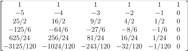
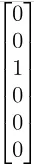
AX = B

X = inv (A) * B

From Matlab,

A = [1 1 1 1 1 1;
    -5 -4 -3 -2 -1 0;
    25/2 16/2 9/2 4/2 1/2 0;
    -125/6 -64/6 -27/6 -8/6 -1/6 0;
    625/24 256/24 81/24 16/24 1/24 0;
    -3125/120 -1024/120 -243/120 -32/120 -1/120 0;];
B = [0;
    0;
    1;
    0;
    0;
    0;];
y = inv(A);
X = y * B

Fig:

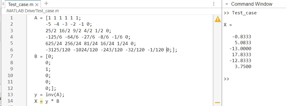
Here, X Stands for unknowns. By equating them,

a = -0.8333

b = 5.0833

c = -13.0000

d = 17.8333

e = -12.8333

g = 3.7500

Substituting these equations,

∂²u/∂x² = [(-0.8333) f (i - 5) + (5.0833) f (i - 4) + (-13) f (i - 3) + (17.8333) f (i - 2) + (-12.8333) f (i - 1) + (3.7500) f (i)]/dx²

----XXXX----XXXX----XXXX----XXXX----

CENTRAL DIFFERENCE SCHEMES:

Nodes are classified as P + Q - 1, so the number of nodes is 5.

EQUATION:

∂²u/∂x² = [af(i - 2) + bf(i - 1) + cf(i) + df(i + 1) + ef(i + 2)]/dx²

From the Taylor series of expansions,

af (i - 2) = [af(i) - [2af' (i) dx/1 + 4af'' (i) dx²/2*1 + 8af''' (i) dx³/3*2*1 + 16af'''' (i) dx⁴/4*3*2*1]]

Table:

dx2 f'' (i)	f (i)	f' (i) dx	f'' (i) dx2	f''' (i) dx3	f'''' (i) dx4
af (i - 2)	a	-2a	2a	-4a/3	2a/3
bf (i - 1)	b	-b	b/2	-b/6	b/24
cf (i)	c	0	0	0	0
df (i + 1)	d	d	d/2	d/6	d/24
ef (i + 2)	e	2e	2e	4e/3	2e/3
Sum of Co-efficients	0	0	1	0	0

In matrix form,

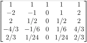
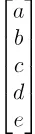
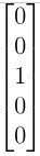
AX = B

X = inv (A) * B

From Matlab,

A = [1 1 1 1 1 ;
    -2 -1 0 1 2;
     2 1/2 0 1/2 2 ;
    -4/3 -1/6 0 1/6 4/3 ;
     2/3 1/24 0 1/24 2/3];
B = [0;
    0;
    1;
    0;
    0];
y = inv(A);
X = y * B

Fig:

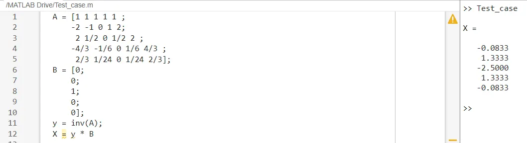
Here, X Stands for unknowns. By equating them,

a = -0.0833

b = 1.3333

c = -2.5000

d = 1.3333

e = -0.0833

Substituting these equations,

∂²u/∂x² = [(-0.0833) f (i -2) + (1.3333) f (i -1) + (-2.5000) f (i) + (1.3333) f (i +1) + (-0.0833) f (i + 2)] / dx²

----XXXX----XXXX----XXXX----XXXX----

MATLAB CODE:

Function code:

RIGHT SKEW SIDED SCHEME

function Error_right_sided_skew = fourth_order_right_sided_skew(x,dx)

% analytical function = exp (x) * cos(x)

% analytical derivative

% f''(x) = -2 *exp (x) * sin(x)

analytical_derivative = -2*exp(x)*sin(x);

% numerical derivative

% central differencing

right_sided_skew = (((3.7500)*((exp(x))*(cos(x))))-((12.8333)*((exp(x+dx))*(cos(x+dx))))+((17.8333)*((exp(x+(2*dx)))*(cos(x+(2*dx)))))-((13.0000)*((exp(x+(3*dx)))*(cos(x+(3*dx)))))+((5.0833)*((exp(x+(4*dx)))*(cos(x+(4*dx)))))-((0.8333)*((exp(x+(5*dx)))*(cos(x+(5*dx))))))/(dx^2);

% error

Error_right_sided_skew = abs(right_sided_skew- analytical_derivative);

end

Function code:

LEFT SKEW SIDED SCHEME

function Error_left_sided_skew = fourth_order_left_sided_skew(x,dx)

% analytical function = exp(x) * cos(x)

% analytical derivative

% f''(x) = -2 * exp(x) * sin(x)

analytical_derivative = -2 * exp(x) * sin(x);

% numerical derivative

% central differencing scheme

left_sided_skew = (((-0.8333)*((exp(x-(5*dx)))*(cos(x-(5*dx)))))+((5.0833)*((exp(x-(4*dx)))*(cos(x-(4*dx)))))-((13.0000)*((exp(x-(3*dx)))*(cos(x-(3*dx)))))+((17.8333)*((exp(x-(2*dx)))*(cos(x-(2*dx)))))-((12.8333)*((exp(x-dx))*(cos(x-dx))))+((3.7500)*((exp(x))*(cos(x)))))/(dx^2);

% error

Error_left_sided_skew = abs(left_sided_skew- analytical_derivative);

end

Function code:

CENTRAL DIFFERENCING SCHEME

function Error_central_differencing = fourth_order_central_differencing(x,dx)

% analytical function = exp(x) * cos(x)

% analytical derivative

% f''(x) = -2 * exp(x) * sin(x)

analytical_derivative = -2 * exp (x) * sin (x);

% numerical derivative

% central differencing

central_differencing = (((-0.0833)*((exp(x-(2*dx)))*(cos(x-(2*dx)))))+((1.3333)*((exp(x-dx))*(cos(x-dx))))-((2.5000)*((exp(x))*(cos(x))))+((1.3333)*((exp(x+dx))*(cos(x+dx))))-((0.0833)*((exp(x+(2*dx)))*(cos(x+(2*dx))))))/(dx^2);

% error

Error_central_differencing = abs(central_differencing- analytical_derivative);

end

Main code:

clear all
close all
clc

% x value

x= pi/3;

% dx range

dx= linspace(pi/4,pi/4000,20);

%for loop
for i=1:length(dx)
    
    central_differencing(i) = fourth_order_central_differencing(x,dx(i));
    
    right_sided_skew(i) = fourth_order_right_sided_skew(x,dx(i));
    
    left_sided_skew(i) = fourth_order_left_sided_skew(x,dx(i));
    
end

%% plot

figure(1)
loglog(dx,central_differencing,'r')
hold on
loglog(dx,right_sided_skew,'g')
hold on
loglog(dx,left_sided_skew,'b')
xlabel('dx range')
ylabel('Truncation error')
title('Range of dx vs Error')
legend('Central differencing','Skewed right sided difference','Skewed left sided difference','location','best')

Fig:

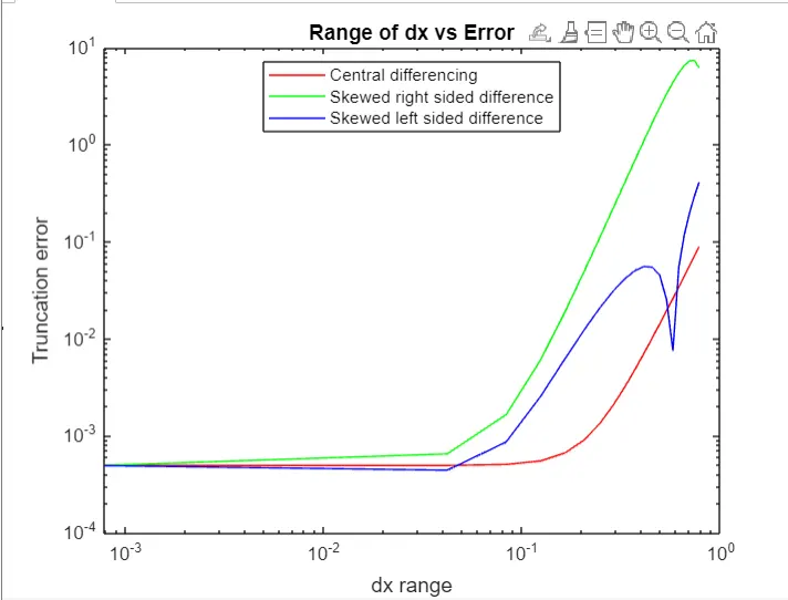
Inference:

• As seen from the plot, the Central differencing scheme is better when compared to other cases.
• The best solution is determined mainly by the errors, which is one of the conditions for choosing the CDS scheme.
• The main reason is that CDS uses information from nodes, which differs from other schemes.
• Cases that don't have information on both sides of CDS fail, and then there comes the Skew scheme to take up the problem.