Aim
Deriving the 4th order approximation in 2nd order derivative using Taylor table method
Objective
Derive the following 4th order approximations of the second-order derivative.
1. Central difference
2. Skewed right-sided difference
3. Skewed left-sided difference
After deriving these schemes, prove that your skewed schemes are fourth-order accurate i.e the thumb rule given in HINT (ii).
Once you have done this, write a program in Matlab to evaluate the second-order derivative of the analytical function exp(x)*cos(x) and compare it with the 3 numerical approximations that you have derived.
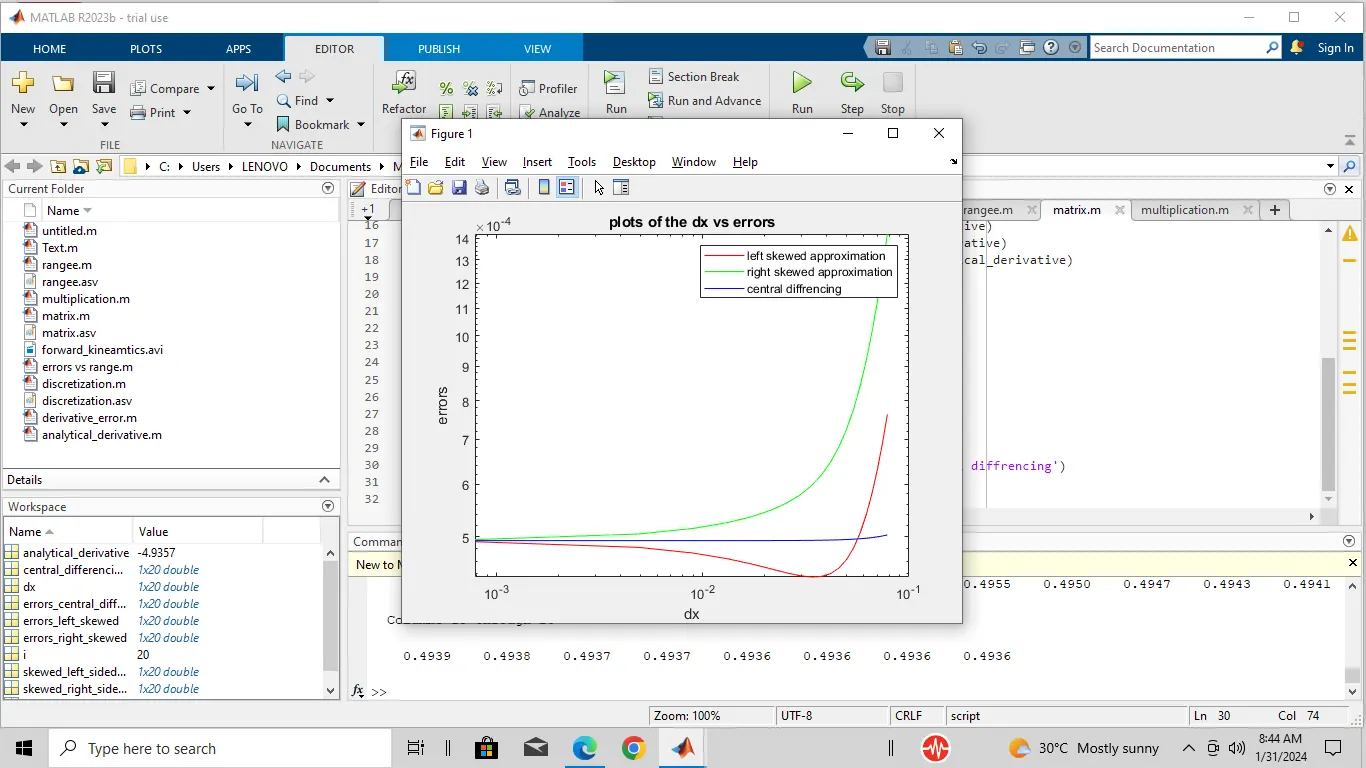
Provide a plot that compares the absolute error between the above-mentioned schemes
In your own words, describe why a skewed scheme is useful? What can a skewed scheme do that a CD scheme cannot?
Explanation
Central diffrencing
Thumb rule is P+Q-1=N
P=Order of accuracy
Q=Order of derivative
N=Number of Stencil
In this scheme P=4,Q=2
N=4+2-1=5
So we take 5 stencil of the discrete points
(△x2)(δ2f
/ δx2 )=a⋅f(i−2)+b⋅f(i−1)+c⋅f(i)+d⋅f(i+1)+e⋅f(i+2)
Using Taylor's Table method
Taylor series
af(i-2)=af(i)-a(f'(i)2.△x)/1!+a(f''(i).4.△x^2)/2!-a(f'''(i)8.△x^3)/6+a(f'''''(i).16.△x^4)/2
Central diffrencing method:
| |
f(i) |
f'(i).△x |
f''(i).4△x^2/2! |
f'''(i).△x^3/6 |
f''''(i)16△x^4/24 |
| af(i-2) |
a |
-2a |
4a/2 |
-8a/6 |
16.a/24 |
| bf(i-1) |
b |
-b |
b/2 |
-b/6 |
b/24 |
| cf(i) |
c |
0 |
0 |
0 |
0 |
| df(i+1) |
d |
d |
d/2 |
d/6 |
d/24 |
| ef(i+2) |
e |
2e |
4e/2 |
8e/6 |
16e/24 |
Matlab code
close all
clear all
clc
x=pi/3;
dx=linspace(pi/40,pi/4000,20);
%analytical derivative=exp*(x).cosx
analytical_derivative=-2*exp(x)*sin(x);
%numerical derivative
for i =1:length(dx)
skewed_left_sided_differencing(i) = (3.75*(exp(x)*cos(x)) - 12.8333*(exp(x-dx(i))*cos(x-dx(i))) + 17.8333*(exp(x-2*dx(i))*cos(x-2*dx(i))) - 13*(exp(x-3*dx(i))*cos(x-3*dx(i))) + 5.0833*(exp(x-4*dx(i))*cos(x-4*dx(i))) - 0.8333*(exp(x-5*dx(i))*cos(x-5*dx(i))))/(dx(i)^2); %skewed left-sided differencing for 2nd order derivative
central_differencing_second_order(i) = (-0.0833*(exp(x-2*dx(i))*cos(x-2*dx(i))) + 1.3333*(exp(x-dx(i))*cos(x-dx(i))) - 2.5*(exp(x)*cos(x)) + 1.3333*((exp(x+dx(i))*cos(x+dx(i)))) - 0.0833*(exp(x+2*dx(i))*cos(x+2*dx(i))))/(dx(i)^2); %central differencing for 2nd order derivative
skewed_right_sided_differencing(i) = (3.75*(exp(x)*cos(x)) - 12.8333*(exp(x+dx(i))*cos(x+dx(i))) + 17.8333*(exp(x+2*dx(i))*cos(x+2*dx(i))) - 13*(exp(x+3*dx(i))*cos(x+3*dx(i))) + 5.0833*(exp(x+4*dx(i))*cos(x+4*dx(i))) - 0.8333*(exp(x+5*dx(i))*cos(x+5*dx(i))))/(dx(i)^2); %skewed right-sided differencing for 2nd order derivative
end
%errors in the approximation
errors_left_skewed=abs(skewed_left_sided_differencing-analytical_derivative)
errors_right_skewed=abs(skewed_right_sided_differencing-analytical_derivative)
errors_central_diffrencing=abs(central_differencing_second_order-analytical_derivative)
%plots
loglog(dx,errors_left_skewed,'color','r','linewidth',0.5)
hold on;
loglog(dx,errors_right_skewed,'color','g','linewidth',0.5)
hold on;
loglog(dx,errors_central_diffrencing,'color','b','linewidth',0.5)
xlabel('dx')
ylabel('errors')
title('plots of the dx vs errors')
legend('left skewed approximation','right skewed approximation','central diffrencing')
Plot
Observation
- It has been concluded that the errors in central differencing method is much less than the other two schemes.
- The left-sided skewed and right sided skewed schemes shows nearly same amount of errors.
Why Skewed scheme is useful?
The skewed scheme is useful because it is necessary to compute the grids at the corners also which central differecing scheme is unable to do. Symmetric nodes does not present on the corners so that CD can not be implemented in such conditions.