Week 3.5 - Deriving 4th order approximation of a 2nd order derivative using Taylor Table method

With the given hint

Order of Accuracy(P)= No of nodes- Order of derivative +1

we calculate the no of nodes to be -> 2+4-1 = 5

so we select the nodes as f(i), f(i-1), f(i+1), f(i-2). f(i+2)

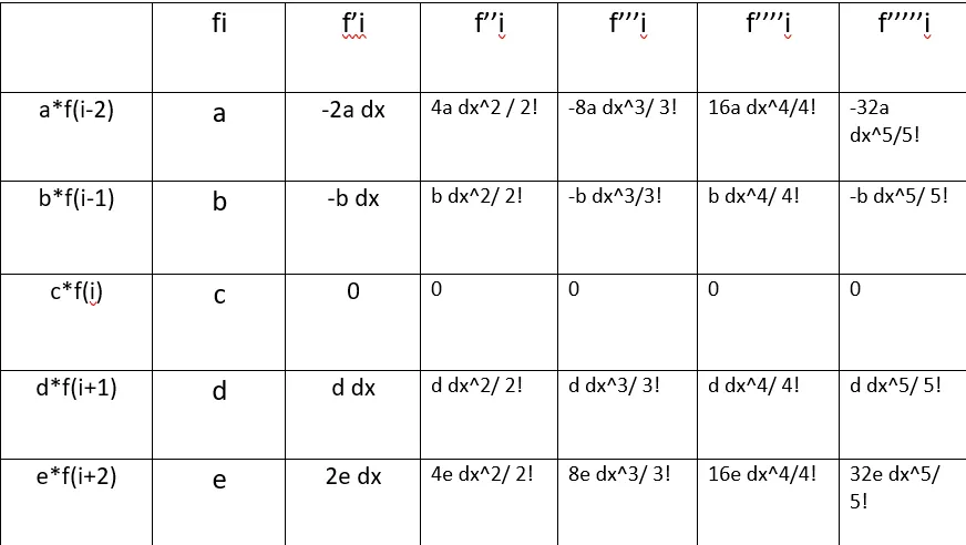
from this, we get 5 equations and 5 unknowns.

The equations are as below:

1. a + b+c+d+e=0
2. -2a dx- b dx+0+d dx+2e dx=0
3. 4a dx^2/ 2! + b dx^2/2! + 0 + d dx^2/2! + 4e dx^2/ 2! =1
4. -8dx^3/ 3! -b dx^3/3! +0 + d dx^3/3! + 8e dx^3/ 3! =0
5. 16 a dx^4/ 4! + b dx^4/ 4!+ 0 + d dx^4/ 4! + 16e dx^4 /4! =0

We equate the third equation to one because we need to find the second derivative.

No, we use a matrix inversion method to solve for a b c d, and e. Putting the coefficients in matrix format, you get

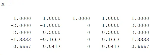
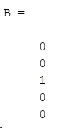
finding the inverse of A ( adjoint A / det A), and multiplying with B, you get the values of a b c d, and e which are

a =-0.08333 b= 1.3333 c=-2.5000 d = 1.3333 e= -0.8333

So the formula is

2. Skewed Right-Sided Difference

Here, in this case, using the formula

Order of Accuracy (P)= Number of Nodes (N) - Order of Derivative Q

so number of nodes = P+ Q = 2 +4 = 6

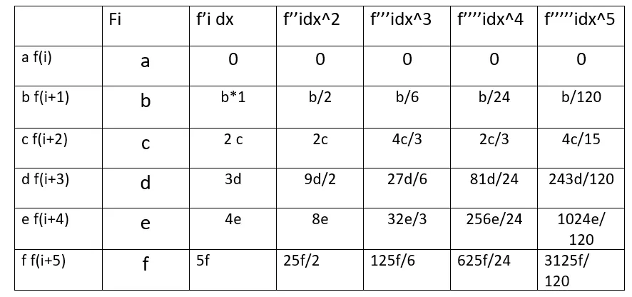
the coefficients in matrix format are given below

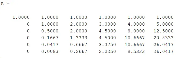
Using the matrix inversion technique, we solve the system of equations and we get the values of a b c d e f as

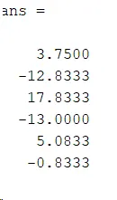
The final equation will be

3. Skewed Left-Sided Difference

We follow the same procedure as we did for the above two

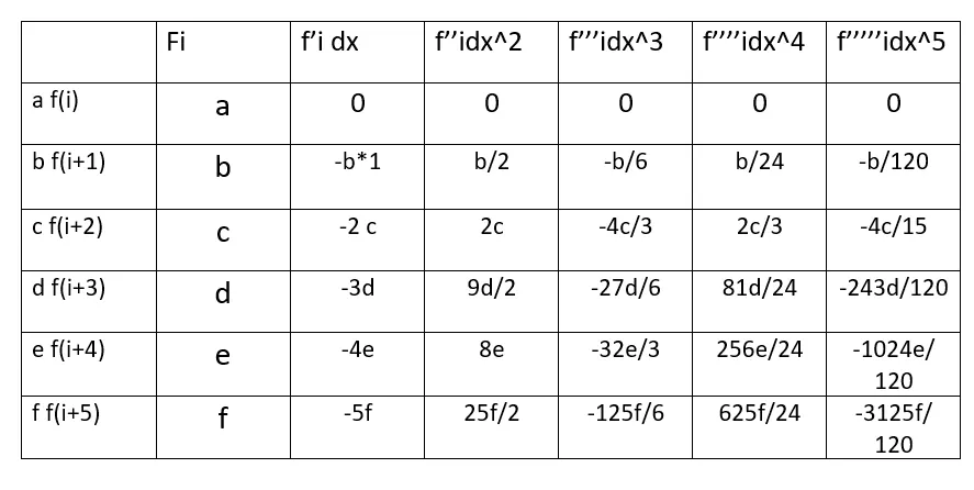
The values remain the same except that the first, third, and 4th derivative terms become negative. After solving using the above methods, you get the values as

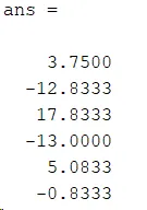
So the final equation is

The schemes have been derived, and now a sample code is run to check which of the schemes gives the most accurate results:

The main code

clear all
close all
clc
% setting the values of dx

dx=linspace(0,pi/4,500);

%setting the value of x

x=pi/3;

for i=1:length(dx)
    
   central_error(i) = cd_function(x,dx(i));
   right_skewed_error(i)=rs_function(x,dx(i));
   left_skewed_error(i)=ls_function(x,dx(i));
   
end

figure(1)
loglog(dx,  right_skewed_error,'linewidth',2)
grid on
hold on
loglog(dx, central_error,'linewidth',2)
xlabel('dx (step size)')
ylabel('absolute error')
grid on
hold on
loglog(dx,left_skewed_error ,'linewidth',2)
legend('4th order right skewed','4th order centrl',' 4th order left skewed')

The functions

1. For the central differencing

function err = cd_function(x,dx)


%analytical derivative of the function e^x cosx
second_derivative = -2*exp(x)*sin(x);

% assigning the matrix
A=[1 1 1 1 1; -2 -1 0 1 2;2 1/2 0 1/2 2 ; -4/3 -1/6 0 1/6 4/3; 2/3 1/24 0 1/24 2/3];
B=[0;0;1;0;0]
C=adjoint(A)/det(A)
inverse= C*B;
values= transpose(inverse)

% formula a f(i-2)+ b f(i-1)+ c f(i)+ d f(i+1)+ e f(i+2)
num_derivative=(((values(1)*(exp(x-(2*dx)))*cos(x-(2*dx))) +(values(2)*(exp(x-dx))*cos(x-dx)) +(values(3)*(exp(x))*cos(x)) +(values(4)*(exp(x+dx))*cos(x+dx)) +(values(5)*(exp(x+(2*dx)))*cos(x+(2*dx)))))/dx^2 ;

%calculating the error
err=abs(second_derivative-num_derivative);


end

2. For left skewed

function err = ls_function(x,dx)


%analytical derivative of the function e^x cosx

second_derivative = -2*exp(x)*sin(x);

% solving for a b c d e f
A=[1 1 1 1 1 1; 0 -1 -2 -3 -4 -5; 0 1/2 2 9/2 8 12.5; 0 -1/6 -4/3 -27/6 -32/3 -125/6 ; 0 -1/24 -2/3 -81/24 -256/24 -625/24; 0 -1/120 -4/15 -243/120 -1024/120 -3125/120]
B=[0;0;1;0;0;0]
C= adjoint(A)/det(A)
inverse= C*B
values= transpose(inverse)



num_derivative=((values(1)*(exp(x)*cos(x))) +(values(2)*(exp(x-dx))*cos(x-dx)) +(values(3)*(exp(x-(2*dx))))*cos(x-(2*dx)) +(values(4)*(exp(x-3*dx))*cos(x-3*dx)) +(values(5)*(exp(x-(4*dx))))*cos(x-(4*dx))+ (values(6)*(exp(x-(5*dx)))*cos(x-(5*dx))))/(dx*dx);

err=abs(second_derivative-num_derivative);


end

3. For Right skewed

function err = rs_function(x,dx)

%analytical derivative of the function e^x cosx
second_derivative = -2*exp(x)*sin(x);
%assigning the matrix
A=[1 1 1 1 1 1; 0 1 2 3 4 5; 0 1/2 2 9/2 8 12.5; 0 1/6 4/3 27/6 32/3 125/6 ; 0 1/24 2/3 81/24 256/24 625/24; 0 1/120 4/15 243/120 1024/120 3125/120]
B=[0;0;1;0;0;0]
C= adjoint(A)/det(A)
inverse= C*B

values=transpose(inverse)


num_derivative=((values(1)*(exp(x)*cos(x))) +(values(2)*(exp(x+dx))*cos(x+dx)) +(values(3)*(exp(x+(2*dx))))*cos(x+(2*dx)) +(values(4)*(exp(x+3*dx))*cos(x+3*dx)) +(values(5)*(exp(x+(4*dx))))*cos(x+(4*dx))+ (values(6)*(exp(x+(5*dx)))*cos(x+(5*dx))))/(dx*dx);

err=abs(second_derivative-num_derivative);


end

PLOTS

The plot given below shows how the step size varies with absolute error for central, left, and right skewed differencing approach.

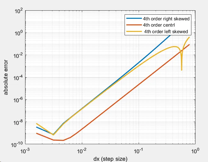
In general, a central scheme is better than a left or right scheme as it takes information from both sides. The accuracy can be better observed from the plot above as the absolute error is lower for the same step size. The main advantage of right / left over a central differencing scheme is that the latter cannot be applied on the boundaries as it takes information from both sides.

-----------------*-----------------------------------*--------------------------------------*-----------------------------------------

(sorry for the late submission, was having trouble with the plots)