Week 3.5 - Deriving 4th order approximation of a 2nd order derivative using Taylor Table method
DERIVING 4th ORDER APPROXIMATION OF A 2ND ORDER DERIVATIVE USING TAYLOR TABLE METHOD
AIM: To write a program for fourth order approximation of 2nd order derivative using central difference, skewed right sided difference, and skewed left sided difference scheme. compare the plot between them.
OBJECTIVE:
<!-- [if !supportLists]-->1. <!--[endif]-->write a program in Matlab to evaluate the second-order derivative of the analytical function exp(x)*cos(x) and compare it with the 3 numerical approximations that you have derived.
<!-- [if !supportLists]-->2. <!--[endif]-->Provide a plot that compares the absolute error between the above-mentioned schemes.
<!-- [if !supportLists]-->3. <!--[endif]-->In your own words, describe why a skewed scheme is useful? What can a skewed scheme do that a CD scheme cannot?
INTRODUCTION:
Central difference scheme:
P = N-Q+1
Where P – order of accuracy,
N – number of nodes,
Q – order of derivative.
N = P+Q-1
N = 4+2-1
N=5
f’’(i) =(a*f(i-2) +b*f(i-1) +c*f(i)+ d*f(i+1) +e*f(i+2))/(h^2)
Expanding each term of the equation using taylor series expansion following is the taylor table of the equation,
| f(x) | f'(x)dx | f''(x)dx2 | f'''(x)dx3 | f''''(x)dx4 | f'''''(x)dx5 | |
| a*f(i-2) | a | -2a | 4a/2 | -8a/6 | 16a/24 | -32a/120 |
| b*f(i-1) | b | -b | b/2 | -b/6 | b/24 | -b/120 |
| c*f(i) | c | 0 | 0 | 0 | 0 | 0 |
| d*f(i+1) | d | -d | d/2 | d/6 | d/24 | d/120 |
| e*f(i+2) | e | 2e | 4e/2 | 8e/6 | 16e/24 | 32e/120 |
| sum of series terms | 0 | 0 | 1 | 0 | 0 | (not required) |
By using matrix inversion method in Matlab to find the coefficient y =inv (A)*B
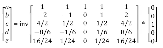
After solving the equation, we get
a= -0.0833, b= 1.3333, c= -2.5000, d= 1.3333, e= -0.0833
By using above condition, we should write a program for central differencing scheme.
Skewed differencing scheme’s:
P = N-Q
Where P – order of accuracy,
N – number of nodes,
Q – order of derivative.
N = P+Q
N = 4+2
N=6
Number of nodes for both skewed right and left sided difference scheme is 6.
Skewed right sided difference scheme:
f’’(i) = (a* f(i)+ b*f(i+1) +c*f(i+2) + d*f(i+3) +e*f(i+4) +j*f(i+5) +k*f(i+6))/(h^2)
Expanding each term of the equation using taylor series expansion following is the taylor table of the equation,
| f(x) | f'(x)dx | f''(x)dx2 | f'''(x)dx3 | f''''(x)dx4 | f'''''(x)dx5 | |
| a*f(i) | a | 0 | 0 | 0 | 0 | 0 |
| b*f(i+1) | b | b | b/2 | b/6 | b/24 | b/120 |
| c*f(i+2) | c | 2c | 4c/2 | 8c/6 | 16c/24 | 32c/120 |
| d*f(i+3) | d | 3d | 9d/2 | 27d/6 | 81d/24 | 243d/120 |
| e*f(i+4) | e | 4e | 16e/2 | 64e/6 | 256e/24 | 1024e/120 |
| j*f(i+5) | j | 5j | 25j/2 | 125j/6 | 625j/24 | 3125j/120 |
| sum of series terms | 0 | 0 | 1 | 0 | 0 | 0 |
By using matrix inversion method in Matlab to find the coefficient y =inv (A)*B
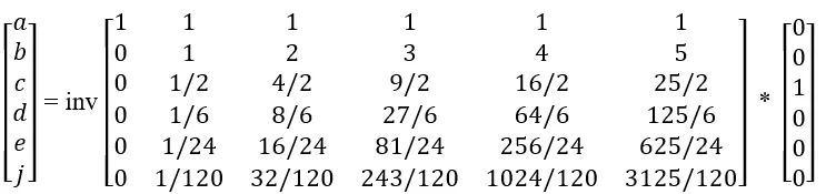
After solving the equation, we get
a= 3.7500, b= -12.8333, c= 17.8333, d= -13.0000, e= 5.0833, j= -0.8333
By using above condition, we should write a program for skewed right sided differencing scheme.
Skewed left sided difference scheme:
f’’(i) = (a* f(i-5) + b*f(i-4) +c*f(i-3) + d*f(i-2) +e*f(i-1) +j*f(i))/(h^2)
Expanding each term of the equation using taylor series expansion following is the taylor table of the equation,
| f(x) | f'(x)dx | f''(x)dx2 | f'''(x)dx3 | f''''(x)dx4 | f'''''(x)dx5 | |
| a*f(i-5) | a | -5a | 25a/2 | -125a/6 | 625a/24 | -3125a/120 |
| b*f(i-4) | b | -4b | 16b/2 | -64b/6 | 256b/24 | -1024b/120 |
| c*f(i-3) | c | -3c | 9c/2 | -27c/6 | 81c/24 | -243c/120 |
| d*f(i-2) | d | -2d | 4d/2 | -8d/6 | 16d/24 | -32d/120 |
| e*f(i-1) | e | -e | e/2 | -e/6 | e/24 | -e/120 |
| j*f(i) | j | 0 | 0 | 0 | 0 | 0 |
| sum of series terms | 0 | 0 | 1 | 0 | 0 | 0 |
By using matrix inversion method in Matlab to find the coefficient y =inv (A)*B
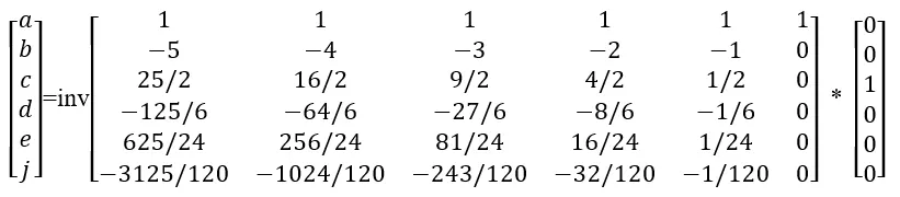
After solving the equation, we get
a= -0.8333, b= 5.0833, c= -13.0000, d= 17.8333, e= -12.8333, j= 3.7500
By using above condition, we should write a program for skewed left sided differencing scheme.
MATLAB CODE:
Function code for central differencing scheme (C_D_S)
function Error_C_D_S = fourth_order_C_D_S(x, dx)A=[1 1 1 1 1;-2 -1 0 1 2;4/2 1/2 0 1/2 4/2;-8/6 -1/6 0 1/6 8/6;16/24 1/24 0 1/24 16/24]B=[0;0;1;0;0]y=inv(A)*B% Analytical derivative%f(x) = exp(x)*cos(x);%f''(x)= -2*exp(x)*sin(x);Analytical_derivative = -2*exp(x)*sin(x)% Numerical derivative�ntral differencing scheme(C_D_S)C_D_S =(y(1)*exp(x-2*dx)*cos(x-2*dx)+ y(2)*exp(x-1*dx)*cos(x-1*dx)+ y(3)*exp(x)*cos(x)+ y(4)*exp(x+1*dx)*cos(x+1*dx)+ y(5)*exp(x+2*dx)*cos(x+2*dx))/(dx^2);% error calculationError_C_D_S = abs(Analytical_derivative-C_D_S);function Error_S_R_S_D = fourth_order_S_R_S_D(x, dx)A=[1 1 1 1 1 1;0 1 2 3 4 5;0 1/2 2 9/2 8 25/2;0 1/6 4/3 9/2 32/3 125/6;0 1/24 2/3 81/24 256/24 625/24;0 1/120 32/120 243/120 1024/120 3125/120]B = [0;0;1;0;0;0]y=inv(A)*B% Analytical derivative%f(x) = exp(x)*cos(x);%f''(x)= -2*exp(x)*sin(x);Analytical_derivative = -2*exp(x)*sin(x);% Numerical derivative% skewed right sided difference(S_R_S_D)S_R_S_D =(y(1)*exp(x)*cos(x)+ y(2)*exp(x+1*dx)*cos(x+1*dx)+ y(3)*exp(x+2*dx)*cos(x+2*dx)+ y(4)*exp(x+3*dx)*cos(x+3*dx)+ y(5)*exp(x+4*dx)*cos(x+4*dx)+ y(6)*exp(x+5*dx)*cos(x+5*dx))/(dx^2);% error calculationError_S_R_S_D = abs(Analytical_derivative-S_R_S_D);function Error_S_L_S_D = fourth_order_S_L_S_D(x, dx)A=[1 1 1 1 1 1;-5 -4 -3 -2 -1 0;25/2 16/2 9/2 4/2 1/2 0;-125/6 -64/6 -27/6 -8/6 -1/6 0;625/24 256/24 81/24 16/24 1/24 0;-3125/120 -1024/120 -243/120 -32/120 -1/120 0]B=[0;0;1;0;0;0]y=inv(A)*B% Analytical derivative%f(x) = exp(x)*cos(x);%f''(x)= -2*exp(x)*sin(x);Analytical_derivative = -2*exp(x)*sin(x);% Numerical derivative% skewed left sided difference(S_L_S_D)S_L_S_D = (y(1)*exp(x-5*dx)*cos(x-5*dx)+ y(2)*exp(x-4*dx)*cos(x-4*dx)+ y(3)*exp(x-3*dx)*cos(x-3*dx)+ y(4)*exp(x-2*dx)*cos(x-2*dx)+ y(5)*exp(x-1*dx)*cos(x-1*dx)+ y(6)*exp(x)*cos(x))/(dx^2);% error calculationError_S_L_S_D = abs(Analytical_derivative-S_L_S_D);MAIN CODE
clear allclose allclc% fourth order approx of a 2nd order derivative using taylor series method% we assume value of x and dxx = pi/3;dx = linspace(pi/4,pi/4000,20);% for each values of dx through its lengthfor i= 1:length(dx)Error_C_D_S(i) = fourth_order_C_D_S(x, dx(i));Error_S_R_S_D(i) = fourth_order_S_R_S_D(x, dx(i));Error_S_L_S_D(i) = fourth_order_S_L_S_D(x, dx(i));end% for plotting the graph between dx and order_of_errorfigure(1)% for plotting Error_C_D_S in loglog scale graphloglog(dx,Error_C_D_S)hold on% for plotting Error_S_R_S_D in loglog scale graphloglog(dx,Error_S_R_S_D)% for plotting Error_S_L_S_D in loglog scale graphloglog(dx,Error_S_L_S_D)% for naming the graph plottitle('dx vs order of error')legend('Error_C_D_S','Error_S_R_S_D','Error_S_L_S_D');% naming the axis of the plotxlabel('dx')ylabel('order of error')CODE EXPLANATION:
First, we calculate the analytical solution for f’’(x) = -2*exp(x)*sin(x)
Using function, each fourth order differencing scheme is derived.
Using matrix inversion method y = inv(A)*B is defined.
Then substitute y values in each deriving equation of fourth order differencing scheme accordingly.
In main code, we assume input values for x and dx [x = pi/3], [dx = (pi/4, pi/4000)] the linspace command is used to specifying the range of dx as 20.
For loop is used to formulate fourth order of differencing scheme functions and (i) is used to store the value of dx array.
Plotting the graph between dx and order of error. loglog scale command is used to plot graph while difficult to compare lines of errors. Plotted dx along x-axis and order of error along y-axis.
OUTPUT AND RESULT DISCUSSION: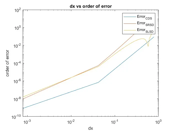
Hence, we conclude that from the graph
Error_S_L_S_D > Error_S_R_S_D > Error_C_D_S
From the results, the central differencing scheme is having lowest error compared to skewed right sided and left sided differencing schemes. While the dx of discretization decreases the order of error also decreases upto some points. Later that there may be increase in order of error.
why a skewed scheme is useful? What can a skewed scheme do that a CD scheme cannot?
Skewed scheme is useful in one directional problem because its take value from either right or left side of the numerical stencil.
For central differencing scheme we need values from both right and left side of the numerical stencil. So, it cannot be used for one direction problems. But for this type of problems skewed scheme gives more accurate values compared to another differencing scheme.
CONCLUSION:
Thus, order of error for central differencing, skewed right sided differencing and skewed left sided differencing is calculated and compared with dx in this challenge. Along with this importance of skewed differencing scheme is studied and applied for an 2nd order derivative.