Week 3.5 - Deriving 4th order approximation of a 2nd order derivative using Taylor Table method

i) Derive the following 4th order approximations of the second-order derivative Central difference, skewed right-sided difference, Skewed left-sided difference by using Taylor table method.

Objective: To evaluate the second-order derivative of the analytical function f(x)= exp(x)*cos(x) using fourth order approximation. And also compare it with the 3 numerical approximations that we have derived. Then, plot that compares the absolute error between the above-mentioned schemes.

The three numerical approximations that we derived are as follows:

Central Differencing Scheme:

Here, the data is taken from both sides of the point that we selected, by using Taylor's method as follows,

(d^2 f)/(dx^2) = af(i-2)+bf(i-1)+cf(i)+df(i+1)+ef(i+2)

Here the no.of =nodes are taken on the bases of type of differencing

Note: for central differencing n=p+q-1
for skewed differencing n=p+q

where, p = order of derivative; q = order of approximation

Therefore, n=2+4-1=5 nodes That means two nodes are selected from both sides of the point that we are focusing.

Then, the Taylors table for central differencing is as follows

coefficients	f(x)	dxf'(x)	dx^2f''(x)	dx^3f'''(x)	dx^4f''''(x)
af(i-2)	a	-2a	2a	-4a/3	2a/3
bf(i-1)	b	-b	b/2	-b/6	b/24
cf(i)	c	0	0	0	0
df(i+1)	d	d	d/2	d/6	d/24
ef(i+2)	e	2e	2e	4e/3	2e/3
sum of the coefficient	0	0	1	0	0

The above equations are transferred into matrix form as AX=B where,

`A=[[1,1,1,1,1] ,[-2,1,0,1,2],[2,1/2,0,1/2,2],[-4/3,-1/6,0,1/6,4/3],[2/3,1/24,0,1/24,2/3]]`

`X=[[a],[b],[c],[d],[e]]` `B=[[0],[0],[1],[0],[0]]`

By solving the above matrix to get the value of x matrix as

X=inv(a)*B

X =

   -0.0833
    1.3333
   -2.5000
    1.3333
   -0.0833

That means a=-0.0833, b=1.3333, c=-2.5000, d= 1.3333, e=-0.0833

These coefficients will further used in code to get the value of derivative.

Skewed right sided differencing:

Here, the data is taken from right sides of the point that we selected, by using Taylor's method as follows,

(d^2 f)/(dx^2) = af(i) + bf(i+1) + cf(i+2) + df(i+3) + ef(i+4) +ff(i+5)

no.of nodes =n=p+q=2+4=6 nodes That refers to 6 nodes are taken from the right side.

Taylor's table for skewed right side differencing

coefficients	f(x)	dx f'(x)	d^2f''(x)	d^3f'''(x)	d^4f''''(x)	d^5f'''''(x)
af(i)	a	0	0	0	0	0
bf(i+1)	b	b	b/2	b/6	b/24	b/120
cf(i+2)	c	2c	4c/2	8c/6	16d/24	32e/120
df(i+3)	d	3d	9d/2	27d/6	81d/24	243d/120
ef(i+4)	e	4d	16e/2	64e/6	256e/24	1024e/120
ff(i+5)	f	5f	25f/2	125f/6	625f/24	3125f/120
sum of coefficients	0	0	1	0	0	0

The above equations are transferred into matrix form as AX=B where,

A=`[[1,1,1,1,1,1],[0,1,2,3,4,5],[0,1/2,4/2,9/2,16/2,25/2],[0,1/6,8/6,27/6,64/6,125/6],[0,1/24,16/24,81/24,256/24,625/24],[0,1/120,32/120,243/120,1024/120,3125/120]]`

`X=[[a],[b],[c],[d],[e],[f]]` B=`[[0],[0],[1],[0],[0],[0]]`

By solving the above matrices to get the value of x matrix as

X=inv(A)*B

X =

    3.7500
  -12.8333
   17.8333
  -13.0000
    5.0833
   -0.8333

That means a=3.7500, b=-12.8333, c=17.8333, d=-13.0000, e=5.0833, f=-0.8333

Skewed left sided differencing:

Here, the data is taken from left sides of the point that we selected, by using Taylor's method as follows,

(d^2 f)/(dx^2) = af(i-5) + bf(i-4) + cf(i-3) + df(i-2) + ef(i-1) +ff(i)

no.of nodes =n=p+q=2+4=6 nodes That refers to 6 nodes are taken from the left side.

Taylor's table for skewed left side differencing:

coefficient	f(x)	dx f'(x)	d^2f''(x)	d^3f'''(x)	d^4f''''(x)	d^5f'''''(x
af(i-5)	a	-5a	25a/2	-125a/6	625a/24	-3125a/120
bf(i-4)	b	-4b	16b/2	-64b/6	256b/24	-1024b/120
cf(i-3)	c	-3c	9c/2	-27c/6	81c/24	-243c/120
df(i-2)	d	-2d	4d/2	-8d/6	16d/24	-32dd/120
ef(i-1)	e	-e	e/2	-e/6	e/24	-e/120
ff(i)	f	0	0	0	0	0
sum of coefficients	0	0	1	0	0	0

The above equations are transferred into matrix form as AX=B where,

A=`[[1,1,1,1,1,1],[-5,-4,-3,-2,-1,0],[25/2,16/2,9/2,4/2,1/2,0],[-125/6,-64/6,-27/6,-8/6,-1/6,0],[625/24,256/24,81/24,16/24,1/24,0],[-3125/120,-1024/120,-243/120,-32/120,-1/120,0]]`

`X=[[a],[b],[c],[d],[e],[f]]` B=`[[0],[0],[1],[0],[0],[0]]`

By solving the above matrices to get the value of x matrix as

X=inv(A)*B

X =

   -0.8333
    5.0833
  -13.0000
   17.8333
  -12.8333
    3.7500

That means a=-0.8333, b=5.0833, c=-13.0000, d=17.8333, e=-12.8333, f=3.7500

ii) Program in Matlab to evaluate the second-order derivative of the analytical function exp(x)*cos(x)

FUNCTION CODE FOR CENTRAL DIFFERENCING:

%function for fourth_order_central_differencing
% error_1 is fourth order central differencing error
function error_1=fourth_order_central_differencing_fun(x,dx)
% f(x)=exp(x)*cos(x)
%f''(x)=-2*exp(x)*sin(x)
analytical_derivative=-2*exp(x)*sin(x);
% central differencing
central_differencing = (((-0.0833)*((exp(x-(2*dx)))*(cos(x-(2*dx)))))+((1.3333)*((exp(x-dx))*(cos(x-dx))))-((2.5000)*((exp(x))*(cos(x))))+((1.3333)*((exp(x+dx))*(cos(x+dx))))-((0.0833)*((exp(x+(2*dx)))*(cos(x+(2*dx))))))/(dx^2);

%error for fourth order central differencing
error_1=abs(central_differencing-analytical_derivative);
end

FUNCTION CODE FOR SKEWED RIGHT SIDED DIFFERENCE:

%function for fourth_order_right_sided_skew
% error_2 is fourth order right sided differencing error
function error_2=fourth_order_right_sided_skew_fun(x,dx)
% f(x)=exp(x)*cos(x)
%f''(x)=-2*exp(x)*sin(x)
analytical_derivative=-2*exp(x)*sin(x);
% skewed_right_sided__differencing
skewed_right_sided__differencing = (((3.7500)*((exp(x))*(cos(x))))-((12.8333)*((exp(x+dx))*(cos(x+dx))))+((17.8333)*((exp(x+(2*dx)))*(cos(x+(2*dx)))))-((13.0000)*((exp(x+(3*dx)))*(cos(x+(3*dx)))))+((5.0833)*((exp(x+(4*dx)))*(cos(x+(4*dx)))))-((0.8333)*((exp(x+(5*dx)))*(cos(x+(5*dx))))))/(dx^2);

%error for skewed_right_sided__differencing
error_2=abs(skewed_right_sided__differencing-analytical_derivative);
end

FUNCTION CODE FOR SKEWED LEFT SIDED DIFFERENCE:

%function for fourth_order_left_sided_skew
% error_2 is fourth order left sided differencing error
function error_2=fourth_order_left_sided_skew_fun(x,dx)
% f(x)=exp(x)*cos(x)
%f''(x)=-2*exp(x)*sin(x)
analytical_derivative=-2*exp(x)*sin(x);
% skewed_left_sided__differencing
skewed_left_sided__differencing = (((-0.8333)*((exp(x-(5*dx)))*(cos(x-(5*dx)))))+((5.0833)*((exp(x-(4*dx)))*(cos(x-(4*dx)))))-((13.0000)*((exp(x-(3*dx)))*(cos(x-(3*dx)))))+((17.8333)*((exp(x-(2*dx)))*(cos(x-(2*dx)))))-((12.8333)*((exp(x-dx))*(cos(x-dx))))+((3.7500)*((exp(x))*(cos(x)))))/(dx^2);

%error for skewed_left_sided__differencing
error_2=abs(skewed_left_sided__differencing-analytical_derivative);
end

MAIN CODE:

clear all
close all
clc
%declaring x and dx
 x = pi/3;
 dx = linspace(pi/40,pi/4000,20);
 for i  = 1:length(dx)
error_1(i)=fourth_order_central_differencing_fun(x,dx(i));
error_2(i)=fourth_order_right_sided_skew_fun(x,dx(i));
error_4(i)=fourth_order_left_sided_skew_fun(x,dx(i));
 end
 plot(error_1,dx,'r',LineWidth=3);
 hold on
 plot(error_2,dx,'b',LineWidth=3);
 hold on
 plot(error_4,dx,'g',LineWidth=3);
 xlabel error
 ylabel dx
 legend('central differencing','skewed right sided differencing','skewed left sided differencing')

Result:

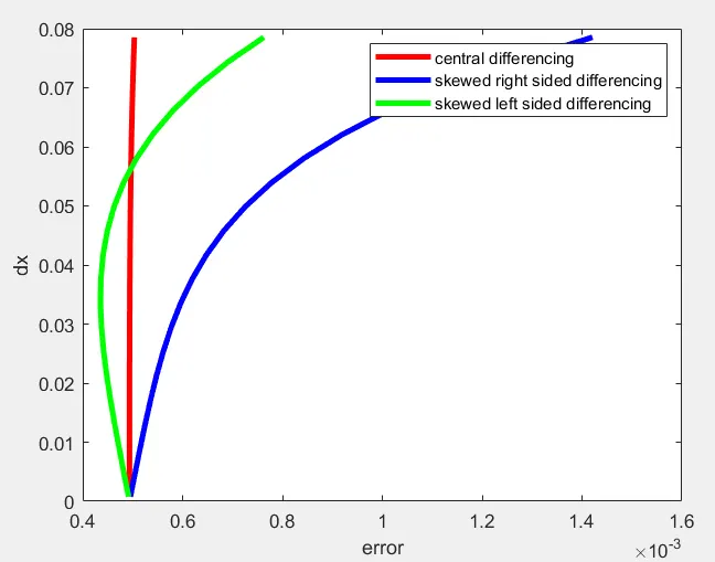
Conclusion:

Here, we plotted the graph between the teuncation error and differencing error of the fourth order differencing approximation and we observe that the central differencing showing less error than others because it uses both the sides node data of our considered node.

Why a skewed scheme is used

When a system that contains only one-sided data either right or left in those cases skewed scheme differencing is used. Here, the skewed scheme depends only on the one side boundary nodes of the system, whereas the central differencing depends on both sides of boundary nodes.